Guide
Window by window
The quick start, demo expectations, inputs and outputs and troubleshooting of every window. The same text is in each window under ? Help.
In every window: work down the numbered step cards on the left (Load → Settings → Run → Save), read the status bar at the bottom, and use Try demo data to check the numbers below. To report a problem, open a GitHub issue with your MATLAB version, the window, what you clicked and the exact message.
Getting started
Launcher
Neuronal Data Analyzer Lab: analysis of blood flow (LDF, laser speckle), electrophysiology, EEG and imaging, step by step. More on this pipeline.
Quick start
- In the launcher, click Set folders and choose your Import folder (raw data) and Export folder (results). You can use one folder for both.
- New here? Open ? Help (top right), pick a window and click Try it with demo data: it opens that window with synthetic data whose answers are known, so you can practise and check your numbers before using your own recordings. The Course and the Virtual lab are coming soon.
- Under Analyses, find the tile for your data (grouped as Blood flow, Electrophysiology, EEG, Imaging and Across techniques) and click its numbered steps in order.
- In every window, work down the numbered step cards on the left: Load → Settings → Run → Save. The teal button is the recommended next action; greyed-out buttons are not possible yet.
- Read the status bar at the bottom of each window: it says what happened and what to do next.
- Stuck? Click ? Help in the window header for its quick start and troubleshooting.
- Many files with the same settings? Use Batch processing in the launcher. To keep an analysis, click Save session… (and Report (PDF)…) in the last step of any window.
Inputs and outputs
In
- Blood-flow recordings from LabChart, AcqKnowledge exports, Spike2, EDF / BDF or a table (LDF)
- Laser speckle images: raw camera frames, contrast or exported perfusion images (.mat, TIFF, video)
- TDT tank / block folder, Intan .rhd / .rhs, Open Ephys binary or legacy folder, NWB 2.x, SpikeGLX, Blackrock or Neuralynx (electrophysiology; TDT needs the TDT MATLAB SDK)
- EEG, raw or cleaned: BrainVision, EDF / BDF, XDF, EEG-BIDS, EEGLAB, FieldTrip or plain .mat, one file per participant
- Image stack .mat, multi-frame TIFF or video (imaging; export other microscope files as TIFF first); still images (histology)
- Any saved result with a time vector and signal (response features)
Out
- Intermediate .mat files that the next step loads (cropped LDF, LDF trials, LFP, MUA)
- Final results: grand averages, ERP/CSD, spike sorting, ROI time series, feature tables (.csv / .mat)
Overview
The launcher
The Learn area: the Course (step-by-step lessons in the real windows) and the Virtual lab (a simulated experiment to plan, record and analyse) are shown with a greyed-out Coming soon button: they are not in this release. ? Help at the top right opens the in-app Help; every window's topic has Try it with demo data.
The Analyses area has one tile per technique, grouped by family in the same order as the website's Analyses menu. Each tile has its steps as numbered buttons (hover one to see which file goes in and out) and a ? that opens its topic here.
| Family | Tile: windows, in order | Starts from | Ends with |
|---|---|---|---|
| Blood flow | LDF: 1 Extract → 2 Process → 3 Average; Laser speckle | A blood-flow recording (LabChart, AcqKnowledge export, Spike2, EDF or a table); laser speckle images (raw, contrast or perfusion) | Trials .mat; grand average (mean ± SD); flow maps, flow per ROI, response map |
| Electrophysiology | LFP: 1 Extract → 2 LFP analysis; MUA: 1 Extract → 2 MUA analysis | TDT tank, Intan, Open Ephys, NWB, SpikeGLX, Blackrock or Neuralynx | ERP, CSD, time–frequency; spike times, clusters, rasters, rates |
| EEG | EEG analysis | Raw or cleaned EEG: BrainVision .vhdr, EDF / BDF, XDF, EEG-BIDS, EEGLAB .set, FieldTrip .mat or plain .mat, one file per participant | ERPs per condition, mean / peak amplitude, scalp maps, statistics, time–frequency |
| Imaging | ROI analysis; Histology / culture | Image stack (.mat or TIFF); still images (TIFF, PNG / JPG, .mat) | Brightness, ΔF/F, kymograph, vessel diameter; cell counts, markers, regions |
| Across techniques | Response features; Batch processing; Sessions and reports | LDF trials, LFP / ERP .mat or any t and y; a folder of files; a saved session | Feature table and group statistics; one summary table and a log; the analysis reopened in its window |
Sessions and reports
- Every analysis window can save a session (inputs with checksums, settings, results, notes), reopen it later, and write a one-page PDF report. See Sessions and reports.
Checks before you use the numbers
- Windows with a Checks tab (LDF Process, Laser speckle, Histology / culture, LFP Analysis, MUA Analysis, EEG Analysis, ROI Analysis and the Groups & statistics tab of Signal Characterization) look at your data and settings and list what they found, one row per check: Result, Topic and Finding. Click a row to read the whole check: what was found, why it matters and what to try. Batch processing puts the checks of each LDF, LFP, MUA and EEG file in a Checks column.
- Blood flow is checked the same way whatever measured it (the needle probe, laser speckle or an imager's perfusion images): baseline drift, movement artefacts, a signal stuck at 0 or at the top, trials left out, short trial baselines and the time resolution; each source adds its own checks.
- Electrophysiology: LFP (a stimulus artefact lasting into the N1 window, the CSD sink at an edge contact, an electrode spacing the file does not give), MUA (spikes closer than the refractory period, a low signal-to-noise ratio, spike amplitudes drifting over the recording) and EEG (trials left per condition, a rejection that hits one condition more, many bad channels, a measured channel that was interpolated).
- Imaging: ROI Analysis (the tissue moving by more than a cell is wide, bleaching, pixels clipped at the camera's top value). Statistics: Groups & statistics (n, and every trial counted as an animal; normality; sphericity with repeated measures; equal spread for ANOVA; whether the parametric and rank-based tests agree).
- The demo files
demo_ldf_faults.mat,demo_lsci_faults.mat,demo_perfusion_faults.mat,demo_lfp_faults.mat,demo_mua_faults.mat,demo_eeg_faults.mat,demo_imaging_faults.matand the foldergroups_faults/contain faults, so you can see each check fire. - OK (green): nothing to do. Check (amber): look at it; it may be fine. Warning (red): the numbers are probably wrong until you fix it. Note (grey): information, such as which model was used.
- The checks are saved in the session, listed on the PDF report (warnings first) and summed up in the methods text.
Typical order
Each step saves a .mat file that the next step loads, so run the steps of a tile from left to right. Signal Characterization comes last: use it on the trials saved by LDF Process or Laser speckle, on the ERP exported by LFP analysis, or on the LFP saved by Extract Ephys, to turn responses into numbers.
Project folders
- Import folder: where Load dialogs start (your raw data).
- Export folder: where Save / Export dialogs start (your results).
- Both are stored as MATLAB preferences (
NeuroAnalyzer.ImportDir,NeuroAnalyzer.ExportDir), so they are remembered between sessions. The launcher asks for them the first time; change them with Set folders.
Requirements
- MATLAB R2021a or later.
- Signal Processing Toolbox: filtering, downsampling and spike detection (LDF Process, Extract Ephys, MUA analysis).
- Image Processing Toolbox: drawing ROIs or a line in ROI analysis and ROIs in Laser speckle (without it, store the ROIs in the .mat file).
- TDT MATLAB SDK: only for Extract Ephys. See README, section "Install the TDT SDK".
The launcher status bar shows whether the Signal Processing Toolbox and the TDT SDK were found.
Where to get help
Every window has a ? Help button that opens its topic here; Learn more opens the matching page of this website, which is also linked at the bottom of every window. To report a bug or ask for a feature, click Report a problem or open https://github.com/alesuarez92/NeuronalDataAnalyzerLab/issues. Include your MATLAB version, the window, what you clicked and the exact message from the status bar or error dialog.
Troubleshooting: 5 common problems
| Problem or message | What to do |
|---|---|
| Undefined function 'Main', 'UIKit' or 'HelpApp' | The toolbox is not on the MATLAB path. Run addpath(genpath('<toolbox folder>')), optionally savepath, then launch with NeuroAnalyzerLab. |
| Launcher warns "Signal Processing Toolbox was not found" | Filtering, downsampling and spike detection will fail. Install it from Home → Add-Ons, or check your license with ver. |
| Extract Ephys: "TDTbin2mat" undefined | The TDT MATLAB SDK is missing. Follow README → "Install the TDT SDK" (place TDTMatlabSDK/ under Utilities/). |
| A file dialog does not appear | It may have opened behind the app window; check the taskbar / Dock. |
| Figures in this help say "not found" | Launch with NeuroAnalyzerLab from the toolbox folder so the docs/ folder can be found. |
LDF pipeline · step 1 of 3
Extract LDF Data
Load a recording (LabChart, AcqKnowledge export, Spike2, EDF or a table), choose the LDF and stimulus, keep the time range of the experiment and save it. More on this pipeline.
Quick start
- 1 Load recording: click Load file... and choose the recording. Check LDF (the flow channel) and Stimulus (a trigger channel, the comments / event markers of the file, or None); both are guessed from the channel names. With several LabChart blocks, choose the Block. The file label shows the format, rate, duration and number of channels.
- 2 Choose time range: type Start and End (s), click Pick on plot and click twice (start, end) on either plot, or click Full range.
- 3 Crop: click Crop to range. The cropped signals replace the full recording in the plots.
- 4 Save: click Save cropped data... and choose a file name. Open this file next in LDF Process.
- Session / report (optional): in step 4, Save session… stores the recording (with checksum), the channels, the range and the crop; Open session… redoes them; Report (PDF)… writes a one-page summary. See Sessions and reports.
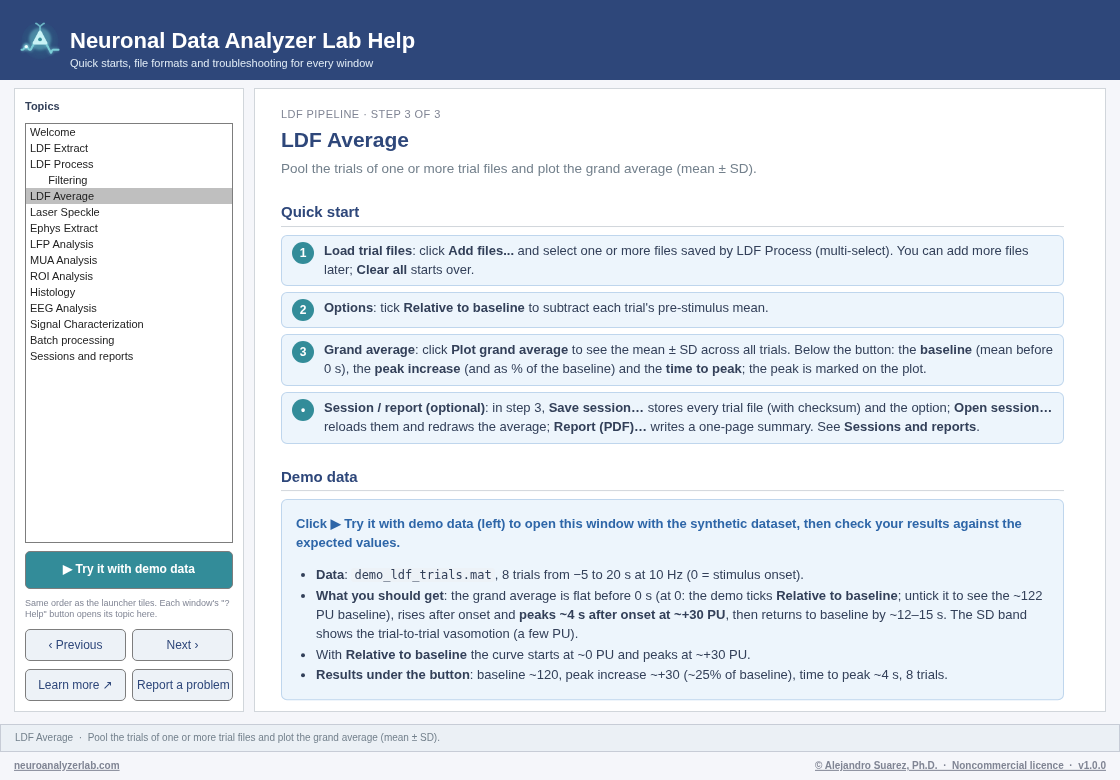
 DEMO DATA — synthetic, generated by core/DemoData.m
Demo data
- Data: LabChart-style export, 8 channels, 300 s at 1000 Hz. Channel 6 = stimulus: 9 pulses of 5 s every 30 s from t = 30 s. Channel 8 = LDF: ~120 PU baseline with slow drift, vasomotion (0.13 Hz), a cardiac ripple (6 Hz) and noise.
- What you should see: after each stimulus pulse the LDF rises by about +30 PU, peaking about 4 s after the onset, and returns to baseline within ~12 s.
- Try: crop 20 to 280 s (this is exactly what the LDF Process demo file contains) and save; the cropped plots start at t = 0 with the first pulse at 10 s.
Inputs and outputs
In
- LabChart (ADInstruments): MATLAB export
.mat(data,datastart,dataend,samplerate,titles,unittext, comments; every block) or text export (.txt) - AcqKnowledge (BIOPAC): its MATLAB export
.mat(data,isi,labels,units) or its text export. Files saved in AcqKnowledge's own format are not read: save the recording as a MATLAB.mator a text file in AcqKnowledge first - Spike2 (CED): MATLAB export
.mat(one struct per channel withtitle,interval,values; event channels withtimes) - EDF / EDF+ / BDF (
.edf,.bdf; LabChart, clinical and many other systems export it): the channels in their physical units; EDF+ annotations can be the stimulus - Tables (
.txt,.csv,.tsv; PeriSoft, moorVMS-PC, spreadsheets): a header row with the channel names (and optionally a units row), a time column in s, ms or clock time; comma, semicolon or tab separated, decimal point or comma. Without a time column the window asks for the sampling rate. - A cropped LDF
.mat(stim,LDF,t,Fs) opens as well - The flow channel is found by its name or units (LDF, flux, perfusion, flow, PU, BPU); the stimulus by its name (stim, trigger, TTL, pulse...) or because it only has two levels. A LabChart file with 8 or more unnamed channels keeps the old convention: stimulus = channel 6, LDF = channel 8.
Out
- Cropped
.matwithstim(stimulus),LDF(flow),t(time in s, 0 at the crop start) andFs(Hz), and the namesflowName,flowUnits,stimName
Troubleshooting: 6 common problems
| Problem or message | What to do |
|---|---|
| "Cannot tell what kind of recording …" / "is not a recording this window knows" | Export the recording as a LabChart or AcqKnowledge .mat, a Spike2 MATLAB export, an EDF file, or a text table with a header row. |
| The LDF or Stimulus dropdown shows the wrong channel | The guess comes from the channel names; choose the right channel in step 1 (name your channels in the acquisition software to make the guess right next time). |
| No stimulus pulses are plotted | Choose the trigger channel, or Comments / markers when the stimuli were marked with comments or event markers. |
| "has no time column" | Type the sampling rate of the rows when asked, or add a first column named Time (s). |
| Sampling rate shows 1000 Hz but the recording used another rate | A LabChart .mat export without samplerate (the status bar warns); re-export with it, otherwise every time axis is wrong. |
| "Start time must be less than End time" / "Range must be within …" | Check the Start and End values (seconds, inside the recording). |
LDF pipeline · step 2 of 3
LDF Processing
Downsample and filter the cropped LDF, cut trials around each stimulus and save them. More on this pipeline.
Quick start
- Load cropped LDF: click Load file... and choose the file saved by LDF Extract.
- Filter / downsample (optional): click Settings..., choose downsampling and filter, click Apply. The Filter response tab shows the filter; Undo returns to the loaded data. See the Filtering topic.
- Segment trials: set Stim threshold (shown as a dashed line on the stimulus), Pre-onset and Post-onset (s) and Min interval (s), then click Segment trials. All trials and the mean ± SD appear in the Trials tab; the Checks tab lists what was checked in the recording and the settings (click a row for why it matters and what to try).
- Save trials: click Save trials.... Choosing an existing trials file appends the new trials to it (time axes must match). Open the file(s) next in LDF Average.
- Session / report (optional): in step 4, Save session… stores the file (with checksum), filter and segmentation settings; Open session… re-runs them; Report (PDF)… writes a one-page summary. See Sessions and reports.
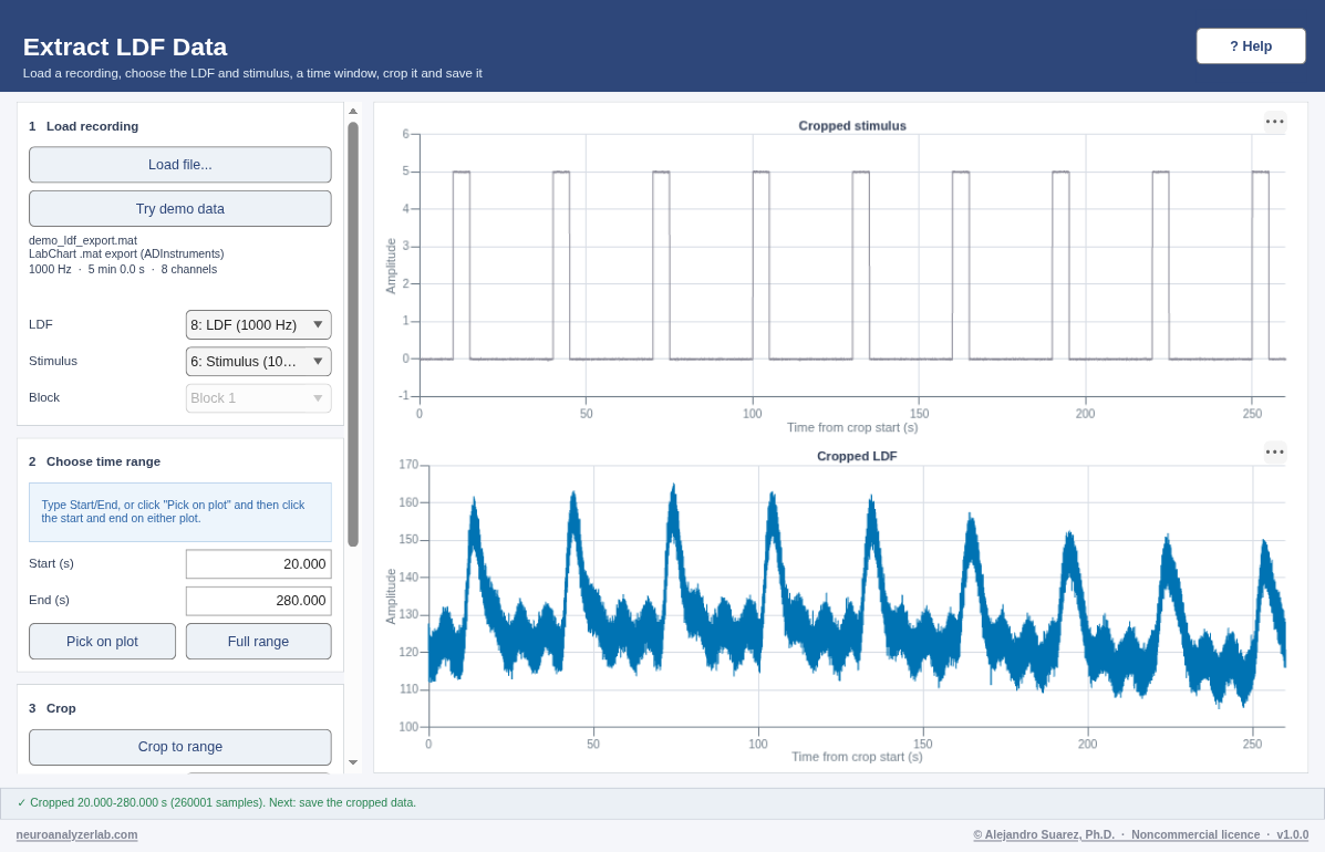
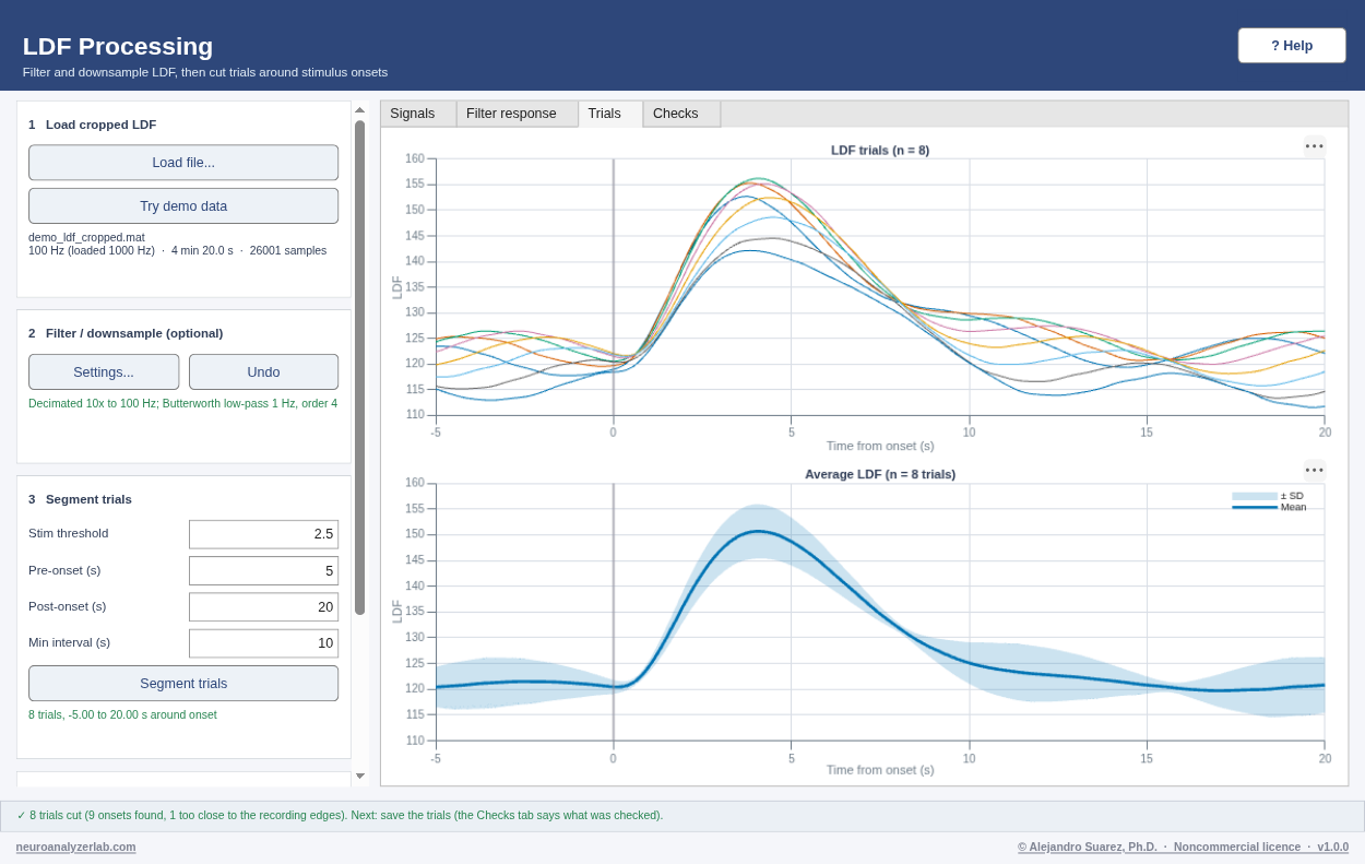 DEMO DATA — synthetic, generated by core/DemoData.m
Demo data
- Data: the cropped demo recording (20–280 s of the LDF export, 1000 Hz): 9 stimulus pulses of 5 s, the first at 10 s, then every 30 s.
- Try: downsample 10x, low-pass ~1 Hz (removes the 6 Hz cardiac ripple), then segment with pre = 5 s and post = 20 s.
- What you should get: 8 complete trials (the last pulse is too close to the end for a 20 s window). The mean response rises after 0 s and peaks ~4 s after onset at ~+30 PU above a ~120 PU baseline.
- Checks: no warnings; one Check, Trials (1 of 9 stimuli left out: its trial does not fit); OK for the baseline (~120 PU), drift (about −1.4%/min from the 8 trial baselines), movement artefacts, signal range, the filter and the time resolution.
- Faults demo: load
demo_ldf_faults.matfrom the demo folder and segment with the same settings: Baseline drift is a Check (about +5.4%/min), Movement artefacts a Warning (jumps at 31 and 72 s, the second in trial 3) and Signal range a Warning (0.38% of the samples at 0).
Inputs and outputs
In
.matfrom LDF Extract withstim,LDF,t,Fs(all four are required)
Out
.matwithsegmentedLDF(trials × samples),segmentedTime(s, 0 = stimulus onset, negative = before) andFs
Troubleshooting: 7 common problems
| Problem or message | What to do |
|---|---|
| "Invalid LDF file. Missing variable(s): …" | Load the file saved by LDF Extract (it contains stim, LDF, t, Fs), not the raw LabChart export. |
| No trials found | The threshold is above the stimulus amplitude or the Min interval is too long. Look at the stimulus plot and lower the threshold. |
| Filter error / cutoff must be below Nyquist | Cutoffs must be below half the sampling rate after downsampling (e.g. 1000 Hz with 10x → Nyquist 50 Hz). |
| Filtering fails with an undefined function (butter, filtfilt, decimate) | The Signal Processing Toolbox is missing (see Welcome → Requirements). |
| "Time axes do not match" when saving | You are appending to a file made with different pre/post times or sampling rate. Save to a new file instead. |
| Checks: movement artefacts in a trial | Look at the times in the Signals tab. Leave those trials out: crop the recording again in LDF Extract, or cut the trials and remove the bad ones before averaging; fix the probe holder for the next recording. |
| Checks: baseline drift | Let the signal settle before the first stimulus (several minutes after placing the probe) and check that the probe holder and the head do not move. A high-pass at 0.02 Hz or below removes slow drift without shrinking the response. |
LDF pipeline · reference
Filtering (reference)
How the digital filters in LDF Process (and Extract Ephys) change a signal. More on this pipeline.
Quick start
- In LDF Process, click Settings (step 2).
- Choose Downsample first: it sets the new sampling rate and therefore the highest usable cutoff (Nyquist = half the rate).
- Pick the filter type and enter the cutoff(s) in Hz; start with order 4.
- Click Apply and compare the filtered trace with the original in the plots; use Undo to try other settings.
Demo data
- Data: the cropped demo LDF (1000 Hz). Besides the ~+30 PU responses it contains a slow drift (period 400 s), vasomotion at 0.13 Hz (±3 PU), a cardiac ripple at 6 Hz (±1.5 PU) and white noise.
- Low-pass 1 Hz (after 10x downsampling): the 6 Hz ripple and most noise disappear, the responses keep their shape and timing (zero-phase filtering: the peak stays ~4 s after onset).
- High-pass 0.2 Hz: removes drift and vasomotion but also shrinks and distorts the slow (~5 s wide) responses, a good example of a cutoff that is too high for LDF.
How the filters work
Filters remove or keep certain frequencies in a signal:
- Low-pass: keeps low frequencies, removes high ones (e.g. smooths noise). One cutoff: frequencies above it are attenuated.
- High-pass: removes low frequencies, keeps high ones (e.g. removes slow drift). One cutoff: frequencies below it are attenuated.
- Band-pass: keeps the band between a low and a high cutoff, e.g. 0.5–5 Hz for LDF.
- Notch: removes a narrow band, e.g. 50 / 60 Hz line noise.
Order: a higher order gives a steeper roll-off (sharper cutoff) but can ring or become unstable; 2–4 is usually enough.
Nyquist: cutoffs must be below half the sampling rate. With downsampling, use the new rate: 1000 Hz / 10 = 100 Hz → cutoffs < 50 Hz.
Design: Butterworth has a flat pass-band; Chebyshev I is steeper but has pass-band ripple; FIR is always stable but needs a high order for a sharp cutoff.
Troubleshooting: 3 common problems
| Problem or message | What to do |
|---|---|
| Cutoff rejected / filter unstable | Keep cutoffs between 0 and Nyquist, low < high for band-pass, and lower the order. |
| The filtered signal looks shifted or distorted at the edges | Edge transients are normal for strong filters; crop a little extra in LDF Extract so trials are away from the edges. |
| Undefined function butter / cheby1 / fir1 | Install the Signal Processing Toolbox. |
LDF pipeline · step 3 of 3
Average LDF Viewer
Pool the trials of one or more trial files and plot the grand average (mean ± SD). More on this pipeline.
Quick start
- Load trial files: click Add files... and select one or more files saved by LDF Process (multi-select). You can add more files later; Clear all starts over.
- Options: tick Relative to baseline to subtract each trial's pre-stimulus mean.
- Grand average: click Plot grand average to see the mean ± SD across all trials.
- Session / report (optional): in step 3, Save session… stores every trial file (with checksum) and the option; Open session… reloads them and redraws the average; Report (PDF)… writes a one-page summary. See Sessions and reports.
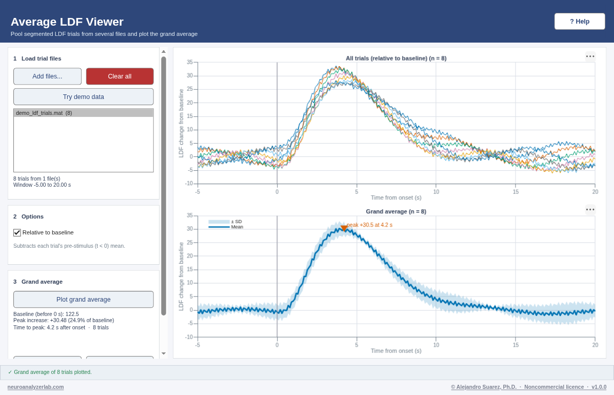 DEMO DATA — synthetic, generated by core/DemoData.m
Demo data
- Data:
demo_ldf_trials.mat, 8 trials from −5 to 20 s at 10 Hz (0 = stimulus onset). - What you should get: the grand average is flat before 0 s (at 0: the demo ticks Relative to baseline; untick it to see the ~122 PU baseline), rises after onset and peaks ~4 s after onset at ~+30 PU, then returns to baseline by ~12–15 s. The SD band shows the trial-to-trial vasomotion (a few PU).
- With Relative to baseline the curve starts at ~0 PU and peaks at ~+30 PU.
Inputs and outputs
In
- One or more
.matfiles withsegmentedLDFandsegmentedTime(from LDF Process, or Save trials… in the Laser speckle window)
Out
- Plots of all trials and of the grand average (mean ± SD); the file list shows how many trials came from each file
Troubleshooting: 3 common problems
| Problem or message | What to do |
|---|---|
| A file was skipped: time axes do not match | Re-segment it in LDF Process with the same pre/post times and downsampling as the other files. |
| A file adds no trials | It does not contain segmentedLDF / segmentedTime; load the file saved by Save trials. |
| "No pre-stimulus baseline available" | The trials start at t = 0. Segment again with pre > 0 s. |
Blood flow · imaging
Laser Speckle Flowmetry
Map blood flow from laser speckle images: the speckle contrast in every pixel, a flow index, the flow in regions over time, the response to each stimulus and where the flow changed. More on this pipeline.
Quick start
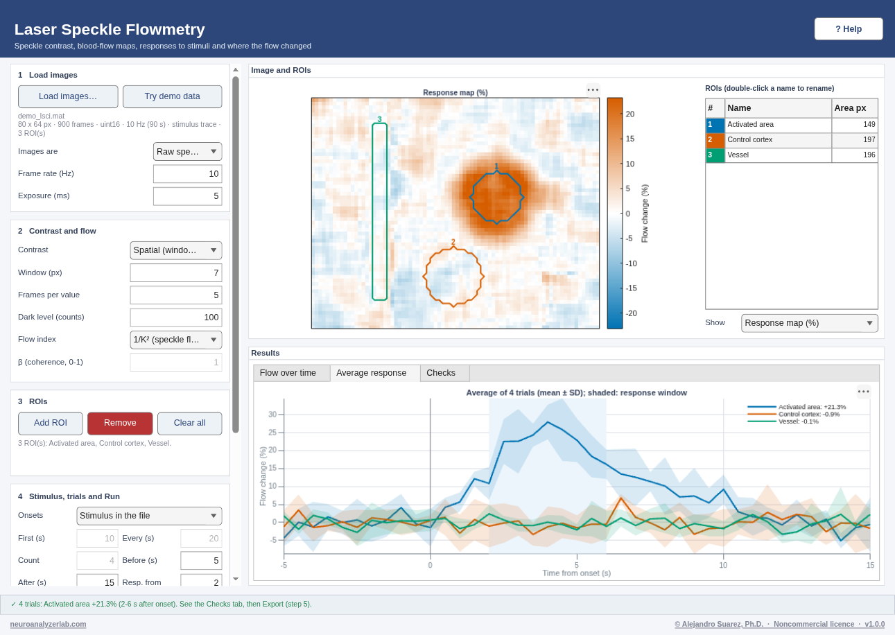
- 1 Load images: click Load images… and choose a .mat (frames H × W × N), a multi-frame TIFF or a video (or Try demo data). Check Images are: Raw speckle images straight from the camera, Speckle contrast (K) images, or Perfusion / flux images already computed by a commercial system (used as they are). Check the Frame rate and, for the 1/τc model, the Exposure (read from the file when it says).
- 2 Contrast and flow (raw images): Spatial contrast in a 7 × 7 window is the usual choice; Frames per value averages the contrast of several frames (set to about 2 values per second when you load). Type the camera Dark level (an image with the laser off). Flow index: 1/K² (the speckle flow index), or 1/τc from the exposure model.
- 3 ROIs: click Add ROI and drag a rectangle over each region (the ROIs of a .mat file are loaded with it). Without ROIs the whole image is one region.
- 4 Stimulus, trials and Run: Onsets from the stimulus trace in the file, a Regular protocol (first onset, interval, count) or None. Before / After set the trial (the part before 0 s is its baseline) and Resp. from / to the response window. Click Run.
- Read the results: Show → Response map (%) colours where the flow rose (orange) or fell (blue); Average response has one curve per ROI (mean ± SD) with its mean change in the response window in the legend; Flow over time the whole recording; Checks lists what to look at before using the numbers (click a row to read why it matters and what to try).
- 5 Export: Export results… writes a .csv (time, flow change % and flow index per ROI) or a .mat (maps, traces, trials, masks, settings); Save trials… writes the trials of the selected ROI in the LDF trial format, which LDF Average and Response features open. Save session…, Report (PDF)… and Methods text… keep the analysis.
 DEMO DATA — synthetic, generated by core/demo/demoLSCI.m
Demo data
- Data:
demo_lsci.mat(or Try demo data): raw speckle images of a rodent cortex, 80 × 64 px (width × height), 900 frames at 10 Hz (90 s), exposure 5 ms, camera dark level 100 counts (uint16). Each pixel is an independent speckle whose contrast follows the exposure model with β = 1. - Tissue: cortex (parenchyma) with τc = T/20 (K = 0.22), a vessel (x = 14–25 px) with τc = T/200 (K = 0.07, much faster flow) and a static corner (bone, K = 0.70, no flow).
- Stimuli: 5 s pulses at 10, 30, 50 and 70 s (
stimin the file). In an activated disk (centre x = 52, y = 28, radius 12 px) the flow rises by 25% at 4 s after each onset and returns within about 12 s; nowhere else does the flow change. - ROIs in the file: Activated area (inside the disk), Control cortex, Vessel.
- Run with the defaults (spatial 7 × 7, 5 frames per value = 2 Hz, dark level 100, 1/K²): 4 trials; Activated area about +21% in the 2–6 s window (the true mean flow change there is +21.9%; 1/K² sees +21.3%), peak about +28% near 4 s; Control cortex and Vessel about 0% (within ±3%). The response map shows an orange disk of about +20% at the activated area and 0 elsewhere.
- Show → Speckle contrast K: cortex 0.22, vessel 0.07 (light), static corner 0.70 (black). The vessel's edges look wider than 12 px because the 7 × 7 window mixes vessel and cortex there.
- Flow index → 1/τc (exposure model): about 4000 /s in the cortex and 40000 /s in the vessel; the activated area rises slightly more than with 1/K² (closer to the true flow change).
- Dark level 0 instead of 100: the contrast drops by about 5% everywhere and Checks has a Check row, Dark level, asking you to measure it; the relative responses hardly change.
- Checks with the defaults: no warnings. One Check, Speckle size (about 1 px): the demo makes each pixel an independent speckle, which a real camera should not do (2 px or more per speckle). Field shift, exposure, illumination, baseline contrast (K = 0.07–0.22), trials, trial baseline (10 samples), time resolution (2 Hz), movement artefacts and signal range are OK; Baseline drift is a Note: 10 s before the first stimulus and 4 trials over 60 s are too short to judge it.
- Faults demo (
demo_lsci_faults.matin the demo folder): Field shift is a Warning (the image moves by up to 4 px, first above 1 px at 46 s); Illumination (−22%), Exposure (25 ms), Baseline contrast (Thinned skull, K = 0.49) and Speckle size are Checks; the contrast is lower everywhere (two speckles per pixel: cortex K = 0.16). - Perfusion demo (
demo_perfusion_faults.mat, opens as perfusion images): Export range is a Warning (13% of the values at 3000 PU: the vessel), Time resolution a Check (one image per second), and three Notes, among them device units and that the dark level, saturation and speckle size checks need raw images. The activated area still rises by about +20%.
Inputs and outputs
In
.matwith the images inframesorstack(H × W × N; any numeric type); optionalt(s per frame) orfps,exposureMs,dark(counts),stim(one value per frame, or a faster trace over the same time),roiMasks(H × W × K logical) withroiNames, andkind('raw speckle', 'contrast' or 'perfusion')- Multi-frame TIFF (raw camera frames or exported perfusion / flux images; the frame interval is read from ImageJ TIFFs) or a video (.avi, .mp4: frame rate from the file; avoid compressed videos for raw speckle)
- Perfusion images from commercial imaging systems (their own files are not read): export them as TIFF, video or MATLAB from the system's software and choose Perfusion / flux images
Out
- .csv:
Time_s, then per ROIFlowChange_pct_<ROI>(change from the baseline window) andFlowIndex_<ROI> - .mat: struct
resultswith the maps (flowMean,K2Mean,responseMap),t,roiFlow,roiRel,trials(ROI × trial × sample, %),trialMean/trialSD,response,peak,peakTime,onsets,checks(lines) andcheckRows(the Checks tab rows), the ROI masks and names and every setting - Save trials:
segmentedLDF(trials × samples, % change of the selected ROI),segmentedTime(s from onset),Fs,onsetTimes,roiName,units: the LDF trial format, for LDF Average and Response features
Troubleshooting: 8 common problems
| Problem or message | What to do |
|---|---|
| The contrast is close to 0 everywhere, or flow index values are huge | The images are probably already processed (perfusion or contrast): set Images are accordingly. |
| The contrast is above 0.6 everywhere | Mostly static tissue, a very short exposure, or speckles much larger than a pixel (close the aperture less / zoom out). Check the focus and the laser. |
| The traces are very noisy | Increase Frames per value (e.g. to one flow value per second), use larger ROIs, or record more stimuli. |
| "Type the frame rate" | The file does not say it: type the Frame rate (Hz) in step 1. |
| Stimuli left out (Checks tab) | Their trial (Before … After) does not fit in the recording; shorten Before / After. |
| Field shift (Checks tab) | The head or the camera moved. Register the frames first (ROI analysis, motion correction) or analyse the part before the shift; fix the head and the camera for the next recording. |
| The response is smaller than expected | With spatial contrast, keep ROIs at least half a window inside the activated area: windows that reach outside mix in unchanged tissue. Try 1/τc with the exposure for large changes. |
| "drawrectangle needs the Image Processing Toolbox" | Save the ROIs as roiMasks (H × W × K) in the .mat with the images. |
Electrophysiology · step 1
Extract Ephys Data
Load a recording (TDT, Intan, Open Ephys, NWB, SpikeGLX, Blackrock, Neuralynx) and extract the LFP and MUA signals for analysis. More on this pipeline.
Quick start
- Load recording: choose the Source (the acquisition system or file format; see Inputs), click Load recording… and select the file or folder it asks for (a TDT tank / block folder, an Open Ephys or Neuralynx folder, or a data file). The channel lists are filled from the recording.
- Choose channels: pick the Stimulus channel (TDT: Whis; Intan: DIGITAL-IN / ANALOG-IN, and the stimulation current in .rhs files; Open Ephys: TTL line / ADC; NWB: stimulus TimeSeries or trials; SpikeGLX: sync or digital bits, analog inputs; Blackrock: analog inputs, digital input bits from the .nev; Neuralynx: TTL bits) and one or more raw channels (All / None help).
- Process: optionally Plot RAW; then Process LFP… (low-pass, optional 60 Hz notch, downsample) and/or Process MUA… (band-pass, default 300–3000 Hz).
- Save: type the probe's Electrode spacing (µm) if you know it (0 = not known; it is saved with the LFP and used for the CSD), then Save LFP… / Save MUA…, choose which channels to keep and a file name (default
<recording>_LFP.mat/<recording>_MUA.mat). Open these files in LFP analysis / MUA analysis. Export NWB… writes the processed LFP and its stimulus channel as an NWB 2.x file (default<recording>_LFP.nwb). - Session / report (optional): in step 4, Save session… stores the recording (with checksum), channels and LFP / MUA settings; Open session… re-processes them; Report (PDF)… writes a one-page summary. See Sessions and reports.
 DEMO DATA — synthetic, generated by core/DemoData.m
Demo data
- Data: a TDT-like demo block (30 s): 8 raw channels (
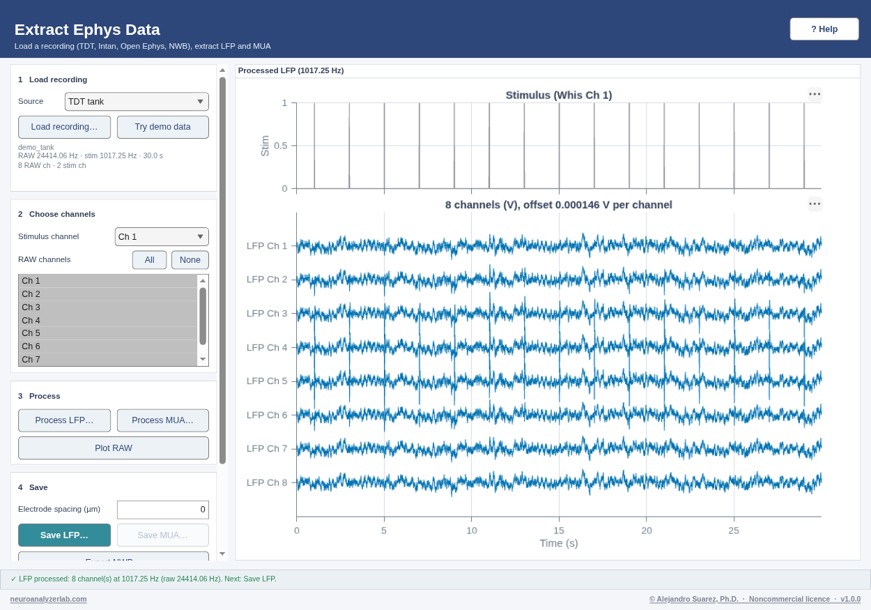
xRAW, 24414 Hz, electrodes 100 µm apart) and the whisker stimulus (Whis: 20 ms pulses every 2 s from 1 s, 15 stimuli). The demo tank is read by a built-in stand-in, so the TDT SDK is not needed for it. - Process LFP (low-pass, downsample to ~1017 Hz): each stimulus evokes a negative deflection at 15 ms and a positive one at 40 ms, largest on channel 4 and weaker with distance from it.
- Process MUA (300–3000 Hz): spikes on channels 3–5 (two units on channel 4, one on channel 5), denser in the 50 ms after each stimulus. Save both to try LFP and MUA Analysis.
- Other formats: choose a Source before Try demo data to open the first 6 s of demo channels 3–6 written as an Intan .rhd (20 kHz; stimulus on DIGITAL-IN-01 and a 1 V copy on ANALOG-IN-1), an Open Ephys folder (30 kHz; TTL line 1 and ADC1) or an NWB file (24414 Hz; the whisker stimulus TimeSeries and a trials table). There are 3 stimuli (1, 3 and 5 s). Process LFP gives 1000 Hz (Intan, Open Ephys) or 1017.25 Hz (NWB), with the evoked negative deflection at 15 ms, largest on RAW Ch 2 (= demo channel 4).
- The same 6 s are also written as SpikeGLX (30 kHz, sync bit 6), Blackrock (.ns6, 30 kHz, NEV digital input bit 0), Neuralynx (32 kHz, TTL bit 0), Intan .rhs (30 kHz, DIGITAL-IN-01) and Open Ephys legacy (30 kHz, TTL 1): the first stimulus candidate is the demo stimulus in each.
- Export NWB… after Process LFP, then choose Source NWB file and Load recording… with the exported file: the LFP opens at its LFP rate with the same channel names and stimulus.
Inputs and outputs
In
- TDT tank / block folder containing the
Whis(stimulus) andxRAW(raw neural) streams (needs the TDT MATLAB SDK,TDTbin2mat, underUtilities/TDTMatlabSDK/) - Intan RHD2000
.rhdfile (file format 1.0–3.x, traditional single-file format) - Open Ephys binary recording folder (GUI 0.5 or later:
structure.oebin,continuous.dat, TTL events) - NWB 2.x
.nwbfile with an ElectricalSeries in /acquisition or /processing - SpikeGLX
.bin+.meta(Neuropixels 1.0 / 2.0 imec AP or LF, nidq) - Blackrock
.ns1–.ns6(NSx 2.1–3.0), with the.nevof the same name for the digital input - Neuralynx folder of
.ncschannels, withEvents.nevfor TTLs - Intan RHS2000
.rhs(stimulation / recording controller, traditional single-file format) - Open Ephys legacy folder:
<processor>_CH<n>.continuousfiles (GUI before 0.6),all_channels.events - Other systems: export the recording from the acquisition software to one of these formats (for example NWB)
Out
- LFP
.mat:lfp_data(channels × samples),lfp_channels,lfp_fs,t_lfp,stim_data,stim_fs,t_stim, andlfp_spacing_umwhen Electrode spacing (µm) is filled in - MUA
.mat:mua_data,mua_channels,mua_fs,t_mua,stim_data,stim_fs,t_stim,filterParams - NWB
.nwb(Export NWB…): LFP in volts in /processing/ecephys/LFP, the stimulus in /stimulus/presentation, electrodes with source channel names. Written with matnwb when installed, otherwise an NWB-style export (not validated).
Troubleshooting: 15 common problems
| Problem or message | What to do |
|---|---|
| "Undefined function TDTbin2mat" or tank does not load | Install the TDT MATLAB SDK: README → "Install the TDT SDK". The folder must be Utilities/TDTMatlabSDK/. |
| "The selected tank does not contain the required Whis and xRAW streams" | Select the block folder of a recording that stored both streams (stimulus as Whis, raw data as xRAW). |
| "Downsample rate must be below the raw rate" | Enter a target rate (Hz) lower than the raw sampling rate shown after loading. |
| Filtering fails (butter, filtfilt, iirnotch undefined) | The Signal Processing Toolbox is missing. |
| Save is disabled | Run Process LFP / Process MUA first; Save stores the last processed result. |
| "not an Intan RHD2000 file: magic number …" | The file is not an Intan .rhd data file. For Intan stimulation files (.rhs) choose Source Intan .rhs. |
| "holds only a header (no data blocks)" | The recording was saved as "one file per signal type" or "one file per channel" (info.rhd + .dat files). Save it in the traditional single-file .rhd format. |
| "… is not a whole number of … data blocks" | The .rhd file is truncated (for example the recording was interrupted). Re-export it from the Intan software. |
| "No structure.oebin found" | Choose the Open Ephys recording folder (…/Record Node */experiment*/recording*) or a folder above it. For the older "Open Ephys format" (.continuous files) choose Source Open Ephys legacy folder. |
| "not an HDF5 file" / "without the NWB root attribute nwb_version" / "No ElectricalSeries" | The file is not an NWB 2.x file with extracellular data. NWB 1.x files are not supported. |
| "Cannot tell the recording format" | Choose the Source yourself before Load recording…; the file may be a format that is not read (for example Blackrock .ccf). |
| The stimulus channel list shows "(no stimulus channel)" | The recording has no digital / analog input, TTL events or stimulus series. LFP / MUA files are still saved, with an all-zero stimulus. |
| Export NWB says "NWB-style file (not validated)" | matnwb is not installed. The file follows the NWB 2.7 layout; install matnwb (https://github.com/NeurodataWithoutBorders/matnwb) to write it with the official schema classes, or validate it with nwbinspector. |
| Loading a long recording runs out of memory | The whole recording is loaded (as for TDT tanks). Split long recordings, or export a shorter segment from the acquisition software. |
Electrophysiology · step 2 (LFP)
LFP / ERP Analysis
Average the LFP around each stimulus (ERP), compute current source density (CSD) and analyse oscillations (spectrum, spectrogram, ERSP / ITPC, band power). More on this pipeline.
Quick start
- Load LFP file: click Load LFP file… and choose the LFP file saved by Extract Ephys.
- Channels: select the channels to analyse (All / None).
- ERP analysis: click Run ERP…, set pre- and post-stimulus time (s), stimulus threshold and minimum ISI (s), click OK. The number of averaged epochs is reported; the Checks tab lists what was checked (click a row for why it matters and what to try).
- CSD: choose the Method (Standard, iCSD delta, iCSD step, iCSD spline or kCSD), enter Spacing (µm) (filled in from the file when it gives
lfp_spacing_um; otherwise type your probe's contact spacing, the default is 100 µm) and the Channel order from top to bottom (at least 3 channels of the last ERP), then click Compute CSD; the Checks tab then also checks the spacing and where the CSD sink lies. iCSD and kCSD also ask for the conductivity σ (S/m) (0.3 for cortex) and the Diameter (µm) of the active tissue (500 by default). iCSD has an optional Smoothing (µm) (0 = off). kCSD has R (µm) and λ, where 0 = chosen automatically by cross-validation. Only the fields of the chosen method are shown (which method?). - Export: click Export ERP / CSD… to save a .mat that Signal Characterization can read.
- Time–frequency: choose the Channel, Frequencies (Hz) (lowest – highest), Wavelet cycles, Epoch (s) and Baseline (s). The band table (delta 1–4, theta 4–8, alpha 8–13, beta 13–30, gamma 30–80 Hz) holds common conventions: edit the limits for your preparation and tick Plot for the bands to show. Try oscillation demo loads a demo with known theta and gamma oscillations and selects channel 4.
- Time–frequency plots (step 6): click Spectrum (power spectrum of the whole recording), Spectrogram (power over time with the stimuli marked), ERSP / ITPC (power change in dB and phase locking around each stimulus) and Band power (% change of each ticked band around the stimulus, mean ± SEM). Each opens its tab. ERSP and Band power use the stimulus onsets found with the ERP threshold (0.5 until you run the ERP).
- Session / report (optional): in step 5, Save session… stores the file (with checksum) and the ERP, CSD and time–frequency settings and results; Open session… re-runs them; Report (PDF)… writes a one-page summary. See Sessions and reports.
 DEMO DATA — synthetic, generated by core/DemoData.m
Demo data
- Data:
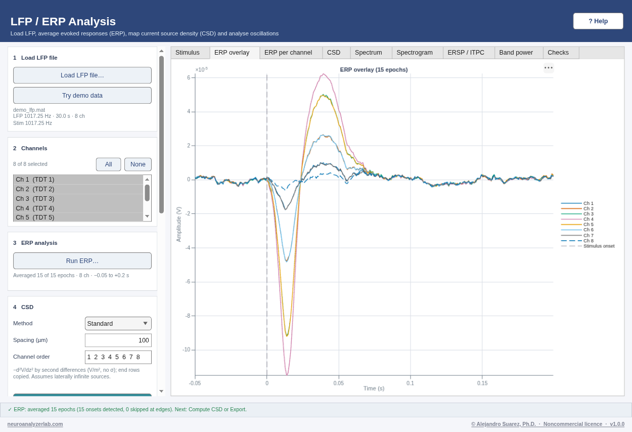
demo_lfp.mat, 8 channels at 1017.25 Hz, 30 s, 100 µm spacing (saved aslfp_spacing_um); 15 stimuli every 2 s from 1 s. - ERP (e.g. pre 0.05 s, post 0.2 s): 15 epochs; N1 (negative) at ~15 ms (about −120 µV at channel 4) and P2 (positive) at ~40 ms; both are largest at channel 4 and fall off over ~150 µm (channels 2–6).
- CSD (spacing 100 µm, order 1–8): a current sink at channel 4 at ~15 ms, flanked by weaker sinks on channels 3 and 5 and by sources further out (channels 1–2 and 6–8).
- Checks (ERP pre 0.05 s / post 0.2 s, then the standard CSD): no warnings and nothing to check. Epochs (15 of 15 stimuli averaged), Stimulus artefact (none), Electrode spacing (100 µm, from the file) and CSD sink (contact 4 of 8, channel 4, inside the probe) are OK.
- Faults demo: load
demo_lfp_faults.matfrom the demo folder with Load LFP file…, select all channels, run the ERP with the same settings and click Compute CSD. Stimulus artefact is a Warning (about +690 µV at the onset, the same on all 8 channels, lasting until about 10 ms: into the N1 window, which starts at 5 ms), Electrode spacing a Check (the file does not give it, so the default 100 µm was used) and CSD sink a Warning (contact 7 of 8 with the standard CSD, contact 8 with iCSD spline: at the edge of the probe, because the response is largest at the deepest contact). - Oscillation demo (Try oscillation demo): the same LFP plus 6 Hz theta (40 µV, on every channel, not phase-locked to the stimuli) and a 40 Hz gamma burst (10 µV, 50–250 ms after each stimulus, channels 3–5, phase-locked). Channel 4 is chosen.
- Spectrum: 1/f background with a clear peak at ~6 Hz (theta) and a small bump near 40 Hz.
- Spectrogram (2–80 Hz): a steady band at 6 Hz, and short 40 Hz patches just after each dashed stimulus line.
- ERSP / ITPC (2–80 Hz, 7 cycles, baseline −0.4 to −0.1 s): about +10 to +12 dB at 36–44 Hz between 50 and 250 ms, ITPC ≈ 0.97 there, and ≈ 0 dB before the stimulus and after ~0.3 s. The ERP itself (N1 / P2) adds a brief broadband increase with high ITPC in the first ~50 ms. On channel 8 (no gamma) there is no 40 Hz increase. 14 of the 15 stimuli are used (the last epoch would run past the end of the recording), and 13 at the lowest frequencies.
- Band power (channel 4): the ERP itself (N1 / P2) gives a very large, brief increase in the first ~50 ms in every band, so the y-axis is scaled to it (the status bar's "largest change" therefore looks from 50 ms on); the gamma burst (roughly +400 to +750 %) is the plateau at 0.05–0.25 s. Theta also swings around the ERP. On channel 8 (far from the ERP, no gamma) theta stays flat (~0 %): theta is not modulated by the stimuli.
Inputs and outputs
In
- LFP
.matfrom Extract Ephys:lfp_data,stim_data,t_lfp,t_stim,lfp_fs,stim_fs(all required); optionallfp_spacing_um, the probe's contact spacing in µm (fills Spacing (µm))
Out
- Tabs: Stimulus (threshold and detected onsets), ERP overlay, ERP per channel (mean ± SD), CSD map
- Export
.mat:t,y(ERP averaged over channels),erp_avg,erp_std,erp_channels,n_epochs,onset_times,erp_params, andcsdwhen computed - Time–frequency tabs: Spectrum (Welch PSD, log–log, bands shaded), Spectrogram (STFT power in dB, dashed stimulus onsets), ERSP / ITPC (dB vs baseline on a blue–white–red scale centred at 0; ITPC 0–1), Band power (% change vs baseline, mean ± SEM per band)
Troubleshooting: 15 common problems
| Problem or message | What to do |
|---|---|
| "Missing variable(s)" when loading | Load the file written by Extract Ephys → Save LFP, not the MUA file or a raw tank. |
| "No stimulus onsets detected. Check the threshold." | Look at the stimulus tab and set the threshold between baseline and stimulus amplitude (the stimulus is mean-subtracted first). |
| "No complete epochs" | All onsets are too close to the recording start / end for the pre/post window. Shorten pre/post. |
| "CSD needs at least 3 channels" / order error | Run the ERP with ≥ 3 channels and list only those channels in the CSD order. |
| "No stimulus onsets detected" in ERSP / ITPC or Band power | These use the ERP stimulus threshold and minimum ISI (0.5 and 0.5 s until the ERP has been run). Run the ERP (step 3) with a threshold that suits the Stimulus tab, then try again. |
| "The highest frequency must be below the Nyquist frequency" | Enter a highest frequency below half the LFP sampling rate (e.g. < 508 Hz for 1017 Hz data). |
| "The baseline window … lies outside the epoch window" | Keep Baseline (s) inside Epoch (s), e.g. epoch −0.5 to 1 s and baseline −0.4 to −0.1 s. |
| ERSP uses fewer trials at low frequencies, or low rows are blank | Low-frequency wavelets are long (3·cycles / (2π·f) s each side); trials whose wavelet would run past the recording start or end are left out at those frequencies. Raise the lowest frequency or use fewer cycles. |
| Band power says n is smaller for delta / theta, or "No epochs far enough from the recording edges" | The band filter needs about 1 s of data on each side of an epoch; trials near the start or end of the recording are left out for that band. |
| A band-table edit is undone | Limits must be numbers ≥ 0 with Low < High; the previous value is restored and the status bar says why. |
| iCSD map is noisy or striped | Inverse CSD amplifies noise between contacts. Set Smoothing (µm) to about 0.5–1 × the spacing (e.g. 50–100 µm), or use kCSD, which chooses its regularisation from the data. |
| CSD values look very different between methods | Standard is in V/m² without the conductivity; iCSD and kCSD are in A/m³ and scale with σ. Compare the depth and timing of sinks and sources, or multiply Standard by σ. |
| Strong sink or source at the top or bottom contact | Activity beyond the ends of the probe is folded into the end contacts (all methods; Standard just copies the neighbouring row). Trust the inner contacts more; kCSD handles this best. |
| Checks: stimulus artefact into the N1 window | Remove the artefact before averaging (blank or interpolate the first milliseconds after each stimulus), or measure the N1 after it (in Batch processing, an N1 window that starts after the artefact). For the next recordings lower the stimulus or use a reference closer to the recording site. |
| Checks: CSD sink at the edge of the probe | The responding layer is at the top or bottom of the probe: next time place the probe so that it lies in the middle of the shank. iCSD spline or step estimate the CSD up to the end contacts; the standard CSD only copies them. |
Electrophysiology · step 2 (MUA)
MUA Analysis
Detect and sort spikes in the MUA signal, check their quality and plot firing rates. More on this pipeline.
Quick start
- Load MUA file: click Load MUA file... and choose the MUA file saved by Extract Ephys. Channels and whether a stimulus is present are shown.
- Channel & segments: choose the channel; optionally tick Segment by stimulation onsets (minimum ISI, threshold, pre / post-stimulus times) and pick a segment.
- Spike sorting: click Configure... (detection method, threshold, polarity, filtering, features, clustering, Auto-merge similar clusters with its Merge threshold (correlation), drift correction) and then Run. With auto-merge on (default), clusters whose mean waveforms have the same shape (correlation ≥ 0.95) and size (amplitude ratio ≥ 0.85) are joined; the status bar says what was merged.
- Clusters: select the clusters to show (Select all / Clear) and read the quality summary. Select two or more units and click Merge selected when they are the same neuron; select one unit and click Split selected to cut it in two; Undo reverses the last merge, split or auto-merge. The Checks tab lists what was checked on the sorted channel (refractory period, signal-to-noise, amplitude drift; click a row for why it matters and what to try) and follows every merge, split and Undo.
- Raster & PSTH tab: spikes of each selected unit (up to 4) around every stimulus onset (raster) and the mean firing rate ± SEM (PSTH). Set From (s), To (s) and Bin (ms); onsets use the threshold and minimum ISI of Segment by stimulation onsets (default 0.5, 1 s).
- Correlograms tab: autocorrelograms (diagonal) and cross-correlograms of up to 4 selected units; set Max lag (ms) and Bin (ms). The shaded band is ± the refractory period: a clean unit has (almost) no spikes there.
- Export: click Save results... to write spike times, cluster IDs, the sorting parameters, quality measures and the list of merges / splits (
info.clusterEdits) to .mat. - Session / report (optional): in step 5, Save session… stores the file (with checksum), all settings and the sorted clusters with your edits; Open session… restores them as saved (Undo still works); Report (PDF)… writes a one-page summary. See Sessions and reports.
 DEMO DATA — synthetic, generated by core/DemoData.m
Demo data
- Data:
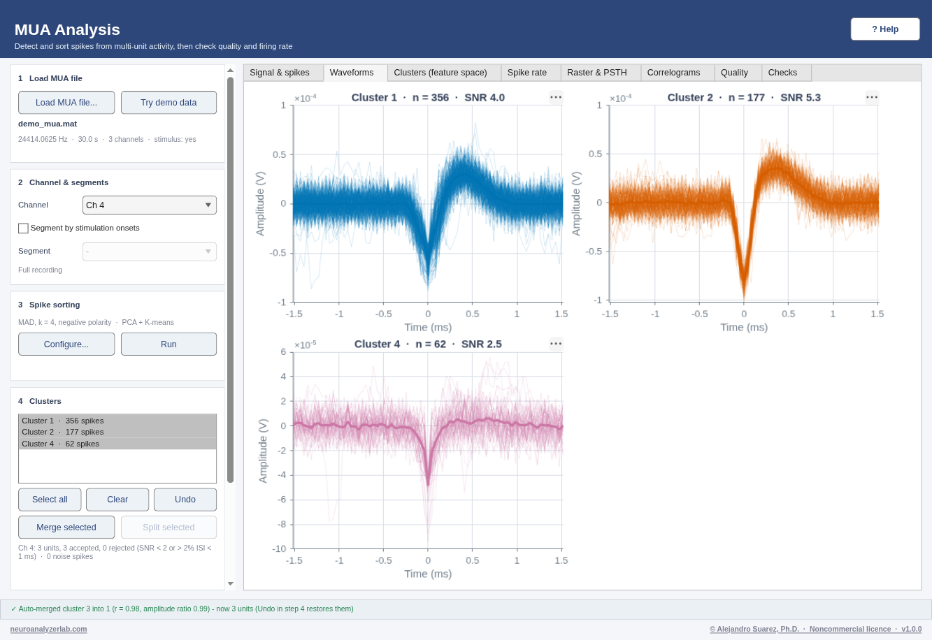
demo_mua.mat, channels 3–5 at 24414 Hz, 30 s, stimulus every 2 s from 1 s. Three units with negative spikes: unit 1 (~90 µV) and unit 2 (~50 µV) on channel 4, unit 3 (~110 µV) on channel 5 (seen weaker on channel 4). Noise ~10 µV. - The demo selects channel 4 and detection MAD, k = 4, negative polarity; click Run.
- What you should get: K-means alone tends to split one unit in two (e.g. 4 clusters, two with the same waveform); with Auto-merge similar clusters on (default) the status bar reports e.g. "Auto-merged cluster 3 into 1 (r = 0.98, amplitude ratio 0.99)" and 2–3 units remain on channel 4: unit 1 (~90 µV), unit 2 (~50 µV) and possibly unit 3 seen weaker from channel 5.
- Raster & PSTH (−0.1 to 0.3 s, 5–10 ms bins): 15 trials; every unit fires more 5–55 ms after each stimulus (unit 1: ~80 vs ~6 spikes/s). Correlograms: the autocorrelograms are empty within ±1 ms (2 ms refractory period); ISI violations ~0%.
- Checks (channel 4): no warnings. Refractory period OK (~0% of intervals under 1 ms), Amplitude drift OK (a few %), Signal-to-noise OK, or a Check when the weak third cluster is kept (unit 3 seen from channel 5 plus noise crossings, SNR ~2.5: close to the noise). Channel 5 is the same (unit 3 SNR ~6.5). Channel 3 has no unit of its own (units 1 and 2 seen from 100 µm, under the threshold): sorting it stops with too few spikes or, when it gives clusters, Signal-to-noise warns, as it should.
- Faults demo: open
demo_mua_faults.matfrom the demo folder with Load MUA file... and run each channel with the same settings. Channel 3 (noise raised to 40 µV): Signal-to-noise is a Warning, no unit reaches SNR 3.5 (about 2.5–2.7). Channel 4 (a ~70 µV unit firing without a refractory period, a quarter of its spikes followed by another 0.8–0.95 ms later): Refractory period is a Check, about 5–8% of that unit's intervals under 1 ms, so it is rejected. Channel 5 (unit 3 shrinks from ~110 to ~55 µV over the 30 s): Amplitude drift is a Warning, about −45%. Signal-to-noise is also a Check there (a small second cluster, SNR ~2.6).
Inputs and outputs
In
- MUA
.matfrom Extract Ephys:mua_data,mua_fs,t_mua,mua_channels - Optional
stim_data,stim_fs,t_stim(needed to segment by stimulus)
Out
- Plots: signal with detected spikes, waveforms, clusters in feature space, spike rate, quality (ISI histograms, alignment check)
- Saved
.mat:SpikeResults(spike times, cluster IDs, waveforms),SpikeSortParams,clusterQuality,info
Troubleshooting: 13 common problems
| Problem or message | What to do |
|---|---|
| "No stimulation data in the loaded file; cannot segment" | The MUA file has no stim_data; save it again from Extract Ephys (it stores the stimulus channel). |
| Very few or no spikes | Lower the threshold multiplier, check the polarity, or enable filtering before detection. |
| Many ISI violations in one cluster | It probably mixes units or noise: try another feature method, more clusters, or a higher threshold. |
| ICA / Wavelet not in the list | They need FastICA or the Wavelet Toolbox; use PCA instead. |
| Detection fails (findpeaks / butter undefined) | Install the Signal Processing Toolbox. |
| Two clusters have the same waveform | One neuron was split: select both and click Merge selected, or turn on Auto-merge similar clusters (Configure...). Lower the Merge threshold (e.g. 0.9) to merge more. |
| Auto-merge joined two different neurons | Click Undo (step 4) to restore the clusters, then raise the Merge threshold (e.g. 0.98) or turn Auto-merge off in Configure.... |
| One cluster mixes two waveforms or has many ISI violations | Select that unit alone and click Split selected; Undo if the result is worse. |
| Raster & PSTH says "No stimulus channel in this file" | The MUA file has no stim_data; save it again from Extract Ephys with the stimulus channel. Correlograms do not need a stimulus. |
| Raster & PSTH says "No stimulus onsets" | The stimulus never rises above the onset threshold: tick Segment by stimulation onsets (step 2) and set a lower threshold, then untick it if you want to sort the full recording. |
| Autocorrelogram has spikes inside the shaded band | The unit has refractory violations: it probably contains a second neuron or noise; try Split selected or a higher detection threshold. |
| Checks: Signal-to-noise warning | The spikes barely cross the threshold. Improve the grounding and the reference, use electrodes of lower impedance or another channel; a higher threshold keeps only the clearest spikes. Report the channel as multi-unit activity at most. |
| Checks: amplitude drift | The electrode moved relative to the neuron: turn on drift correction (Time binning) in Configure..., analyse the stable part (Segment by stimulation onsets), and let the probe settle for several minutes before recording. |
Imaging
ROI / Image Analysis
Measure a ROI or a line over time in a stack of coregistered frames (2-photon, gCaMP, blood-flow imaging). More on this pipeline.
Quick start
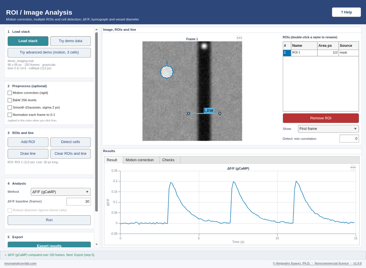
- Load stack: click Load stack and choose a .mat or multi-frame TIFF (or Try demo data / Try advanced demo (motion, 3 cells)). The first frame is shown with the size, frame count and time source; a
roiMask/roiMasksin the file becomes the first ROI(s). - Preprocess (optional): tick Motion correction (rigid) if the frames jitter: the shifts are estimated once (max shift shown next to the box, per-frame plot in the Motion correction tab) and applied before everything else. Then optionally B&W 256 levels, Smooth and/or Normalize each frame, applied in that order when you click Run.
- ROIs and line: click Add ROI and drag a rectangle (repeat for more ROIs), or Detect cells to add one ROI per active cell automatically. ROIs are listed next to the image (double-click a name to rename, Remove ROI to delete). For line methods click Draw line (across the vessel for diameter). Clear ROIs and line starts over.
- Analysis: choose the Method (for ΔF/F also the baseline frames; for Vessel diameter optionally Robust diameter (ignore blood cells)) and click Run. ROI methods give one trace per ROI, in the ROI's colour. The Checks tab (next to Result and Motion correction) lists what was checked: movement against the size of the cells, bleaching and clipped pixels; click a row for why it matters and what to try. The status bar says when there are warnings.
- Export: click Export results to save a .csv (time + one column per measure and ROI) or a .mat (all series, ROI masks and names, line, shifts and settings).
- Session / report (optional): in step 5, Save session… stores the stack (with checksum), ROIs, line and settings; Open session… re-runs motion correction and the analysis; Report (PDF)… writes a one-page summary. See Sessions and reports.
 DEMO DATA — synthetic, generated by core/DemoData.m
Demo data
- Data:
demo_imaging.mat, 96 × 96 px, 150 frames at 10 Hz (15 s). A dark vertical vessel at x = 60 whose diameter oscillates 12 ± 3 px (9–15 px) every 5 s; a bright red blood cell moving down 2 px/frame (20 px/s); a cell at (24, 30), radius 6 px with calcium transients (ΔF/F ≈ 1) at 3, 7 and 11 s. The cell'sroiMaskis in the file. - The demo selects ΔF/F with that mask (baseline = first 30 frames) and a line across the vessel from (45, 70) to (75, 70).
- ΔF/F: flat ~0 until 3 s, then three peaks of ~0.2–0.3 at 3, 7 and 11 s, each decaying in ~1–2 s. (The simulated calcium signal has ΔF/F ≈ 1, but it is added on top of the tissue background inside the ROI, so the measured ΔF/F of the ROI is smaller.)
- Vessel diameter (same line): a sine between ~9 and ~15 px with a 5 s period. Kymograph along the vessel (e.g. from (60, 5) to (60, 90)): slanted streaks with a slope of 2 px per frame.
- Advanced demo (Try advanced demo (motion, 3 cells)): 96 × 96 px, 150 frames at 10 Hz. Every frame is shifted by up to ±3 px (smooth random walk); three cells: cell 1 at (22, 24) with events at 4, 8.5, 13 s, cell 2 at (26, 78) at 5.5, 10.5 s, cell 3 at (82, 30) at 7, 12 s; the vessel at x = 60 (12 ± 3 px, period 5 s) and a bright red blood cell that crosses the diameter line (35, 64)–(85, 64) about every 3 s.
- Motion correction: the Motion correction tab shows dy and dx following the dashed true shifts (error < 0.3 px), max shift ≈ 3 px.
- Show → Correlation image: the three cells are bright disks (correlation ≈ 0.9), the vessel a bright band; Detect cells adds exactly Cell 1–3 (the vessel is rejected as too elongated).
- ΔF/F (Run): three traces, each peaking only at its own cell's event times.
- Vessel diameter: without Robust diameter the trace jumps to ~50 px whenever the blood cell crosses the line; with Robust diameter it follows the 9–15 px sine (error < 2.5 px) and the replaced frames are circled.
- Checks (demo, ΔF/F): no warnings and nothing to check. Motion OK (the frames move by about 0.1 px; the ROI is 12 px across), Bleaching OK (the baseline changes by about 1%), Saturation OK (no ROI pixel clipped).
- Faults demo: load
demo_imaging_faults.matfrom the demo folder with Load stack (its three ROIs, Cell 1–3, come with it), choose ΔF/F (baseline 30 frames) and click Run. The Checks tab gives 3 warnings: Motion (the frames move by up to about 7 px from their usual place, about 70% of a 10 px cell, and motion correction is off), Bleaching (the baseline is about 30% darker at the end than at the start) and Saturation (about 2% of Cell 2's pixels over the recording are at 4095, the top of a 12-bit camera). Tick Motion correction and Run again: Motion becomes OK (frames moved by up to 7 px and were shifted back); bleaching and clipping stay, because they are in the light the camera recorded.
Inputs and outputs
In
.matwithstackorframes(H × W × N grayscale or H × W × 3 × N RGB; otherwise the first variable is used)- Optional in the .mat:
timeVecort(one time per frame),roiMask(logical H × W) orroiMasks(H × W × K, optionalroiNames), used as the first ROIs - Multi-frame TIFF: RGB frames are converted to grayscale (mean of the colour channels). The frame interval, pixel size and channels are read from ImageJ, OME-TIFF and ScanImage files (one channel and the first slice are used); otherwise time = frame index
- Video (
.avi,.mp4): grey frames and the frame rate of the file - Files saved by microscope software in its own layout are not read: export the recording as a multi-frame TIFF (or a video) with that software first
Out
- .csv:
Time_splus one column per measure and ROI (<measure>_<ROI name>, e.g.DFF_Cell_1; measures Intensity, Movement, DFF), orDiameter_px(+Diameter_standard_px,Replacedwhen robust); for a kymograph, a matrix (first row = time) - .mat: struct
resultswith the series (one row per ROI),roiMasks/roiNames,roiMask(ROI 1),lineStart/lineEnd,motionCorrectionandshifts, and the preprocessing and diameter settings
Troubleshooting: 14 common problems
| Problem or message | What to do |
|---|---|
| "Could not draw a rectangle / line" | drawrectangle / drawline need the Image Processing Toolbox. Without it, save a logical roiMask in the .mat for ROI methods. |
| Run is disabled | The chosen method needs a ROI (Brightness, Movement, Both, ΔF/F) or a line (Kymograph, Vessel diameter); the step 3 card says which is missing. |
| "roiMask size does not match" | The mask must be H × W, the same size as one frame. |
| Time axis shows frames, not seconds | Add a timeVec (or t) with one value per frame to the .mat. |
| Load is slow / out of memory | Large TIFFs are read frame by frame into memory as double; crop or bin the stack first. |
| Detect cells finds nothing | Tick Motion correction first: residual motion makes every edge look correlated and raises the automatic threshold. Otherwise lower Detect: min correlation (e.g. 0.3; 0 = automatic). |
| Detect cells also picks up vessels or blobs at the border | Elongated structures (ratio > 3) and components outside 20–1000 px are rejected; after motion correction the border within the largest shift is ignored. Remove unwanted ROIs with Remove ROI. |
| Two touching cells become one ROI | Raise Detect: min correlation so they separate, or draw them with Add ROI. |
| Checks: motion larger than a cell | Tick Motion correction (step 2) and Run again. If the Motion row stays a Check or Warning after it, the tissue bends or moves in depth: analyse a calmer stretch, or correct the movie non-rigidly in another program (e.g. NoRMCorre, suite2p) before loading. |
| Checks: bleaching | Lower the light or the exposure in the next recording; compare responses at the same time in the recording; or correct the bleaching before ΔF/F (divide by an exponential fitted to the baseline). |
| Checks: saturation | The brightest cells are clipped at the camera's top value. Lower the gain, the exposure or the light; leave out the clipped ROIs. |
| Vessel diameter jumps for single frames | A bright blood cell crossing the line moves the half level. Tick Robust diameter (ignore blood cells); make the line extend at least one vessel radius beyond each wall so its ends sample the background. |
| Motion correction shifts look noisy / wrong | It corrects translation only (not rotation or warping) and needs structure in the image; very dim or uniform stacks give unreliable shifts. Untick it to go back to the raw frames. |
| ROIs are slightly off after turning motion correction on or off | ROIs and the line keep their pixel positions; re-run Detect cells or redraw them on the image you analyse. |
Imaging · still images
Histology / culture
Count cells in still images of sections or cultures, find the cells positive for a marker, compare regions, and align sections or time points. More on this pipeline.
Quick start
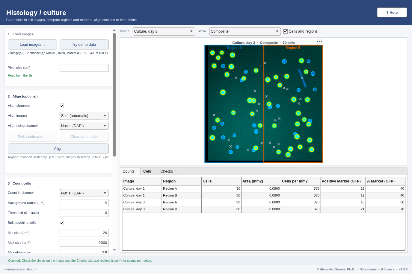
- 1 Load images: click Load images… and choose one or more files (or Try demo data). TIFF: every page is a channel; PNG / JPG: the colours are channels; .mat: variable
images(H × W × channels × images). Several files = several sections, time points or wells, with the same channels. Check the Pixel size (µm): it is read from ImageJ TIFFs; otherwise type the value of your microscope. - 2 Align (optional): tick Align channels if the colours of one cell do not sit on top of each other. With several images choose Align images: Shift (automatic) for the same field imaged again (time points), Landmarks (click points) for serial sections: click Pick landmarks…, click the same 3 or more features in image 1 and in the image shown, then Finish (Clear landmarks starts again). Click Align and switch images to check the overlay.
- 3 Count cells: choose the channel in which every cell is visible (usually nuclei). The defaults suit nuclei of about 8–12 µm; click Count cells. Circles mark counted cells, grey × marks objects that were not counted. Switch Show to What was thresholded to see what counted as cell.
- 4 Regions and markers: every other channel is a marker; a cell is positive when at least Positive if (% of cell) of it is bright in that channel (yellow circles = positive for every marker). Click Add region, click the corners on the image, then Finish, to get counts and densities per region. Import regions… adds regions drawn in ImageJ / Fiji (a
.roi, or the ROI Manager'sRoiSet.zip) or QuPath (annotations exported as GeoJSON), in the pixels of image 1; lines and points are skipped. - 5 Export: Export results… writes a .csv with one row per cell plus
<name>_counts.csv(per image and region), or a .mat with everything. Save session…, Report (PDF)… and Methods text… keep the analysis. - Read the Checks tab before using the numbers: it says where the pixel size came from, how well the images and channels were aligned, which threshold was used and what was left out. Click a row to read why it matters and what to try.
 DEMO DATA — synthetic, generated by core/demo/demoHistology.m
Demo data
- Data:
demo_histology.mat(or Try demo data): two images of the same culture field, Culture, day 1 and Culture, day 3, 400 × 400 px at 1 µm per pixel (0.16 mm²). Channel 1 Nuclei (DAPI), channel 2 Marker (GFP). - 60 nuclei in each image (48 single and 6 touching pairs): 30 in the left half and 30 in the right half. Count cells should give 60 in both images (375 cells per mm²); the pairs are split into two cells each.
- Marker-positive: 24 of 60 on day 1 and 39 of 60 on day 3 (every day-1 positive cell stays positive).
- Not counted: 20 small specks of debris (under 15 µm², removed by Min size) and 1 long fibre (removed by Max elongation). Uneven illumination is removed by the background step.
- Alignment: day 3 was imaged after the dish went back on the stage, shifted by 6.4 px down and 9.2 px left ([dy dx] = [6.4 −9.2]); Shift (automatic) recovers it to about 0.2 px. The marker channel is shifted by [1 2] px from the nuclei in both images (Align channels corrects it).
- Regions: add Region A = left half (x ≤ 200.5) and Region B = right half: 30 cells each (375 per mm², 0.08 mm² each). Marker-positive per region: 12 and 12 on day 1, 18 and 21 on day 3 (after aligning). Without aligning, the Checks tab has a Warning row, Alignment: the regions cover different tissue in the two images (what to try: align them in step 2).
- Checks tab (aligned, default settings): pixel size read from the file; image 2 moved by about 9.2 px right and 6.4 px up; the marker channel was about 2.6 px off (corrected; listed as a row to check, so look at the composite: markers should sit on their nuclei); 20 small objects and 1 elongated object not counted; 6 extra cells found by splitting the touching pairs. Click the Channels row: "What to try: Check the composite: markers should sit on their nuclei."
Inputs and outputs
In
- TIFF (.tif / .tiff): every page is a channel (one RGB page: its colours); the pixel size is read from ImageJ (also µm), OME-TIFF, Aperio .svs or the resolution tags when present
- PNG, JPG, BMP: the colour channels (a grey image is one channel); type the pixel size
- .mat:
images(H × W × C × N) orimage(H × W × C); optionalchannelNames,imageNames,pixelSizeUm - Several files at once: one image each (sections, time points, wells), all with the same channels and size
Out
- .csv: one row per counted cell: image, cell number, x and y (µm), area (µm²), elongation, region, and for every marker positive yes / no and the part of the cell that is bright (%)
<name>_counts.csv: one row per image and region: cells, area (mm²), cells per mm², positive cells and % per marker, cells positive for all markers- .mat: struct
resultswith the same tables, the settings (µm units), regions, alignment (shifts, landmarks, errors), the label images and the per-cell marker values
Troubleshooting: 8 common problems
| Problem or message | What to do |
|---|---|
| Two cells counted as one | Strongly overlapping nuclei (no narrow waist between them) stay one object by design. Make sure Split touching cells is ticked; for dense tissue lower Max size so the Checks tab lists the clumps, and count them by eye. |
| One cell counted as two | Irregular or dividing nuclei can have two distance peaks. Raise Background radius (a too small radius cuts cells) or untick Split touching cells for sparse cultures. |
| Densities (per mm²) look wrong | The pixel size is probably wrong. The Checks tab says whether it came from the file or was typed; for PNG / JPG it must be typed (µm per pixel of your objective and camera, including binning). |
| Background counted as cells, or dim cells missed | Switch Show to What was thresholded: red is what counts as cell. Type a Threshold (0 = automatic) and count again; the Checks tab gives the automatic value to start from. |
| Debris or fibres are counted | Raise Min size (µm²) or lower Max elongation. A round nucleus of 8 µm is about 50 µm²; elongation 1–1.5. |
| Marker calls look wrong | Check that the marker sits on its nucleus in the Composite view; if it is offset, tick Align channels and click Align. Then adjust Positive if (% of cell) or Marker threshold. |
| "Load images with the same channels together" | All images of one analysis need the same number of channels (and the same size). Load images with different stainings separately. |
| Automatic shift unreliable (Checks tab) | The images may show different fields, or be rotated: use Landmarks (click points) instead. |
EEG
EEG Analysis
Clean raw recordings (bad channels, filters, re-reference), cut them into trials and reject the noisy ones, then average the trials of each condition, look at the ERPs, measure a component (mean or peak amplitude in a time window) and map it over the head, compare conditions across participants and look at the time–frequency of each condition (ERSP, phase locking, band power). EEG already cleaned in EEGLAB, FieldTrip or MATLAB is read as it is. More on this pipeline.
Quick start
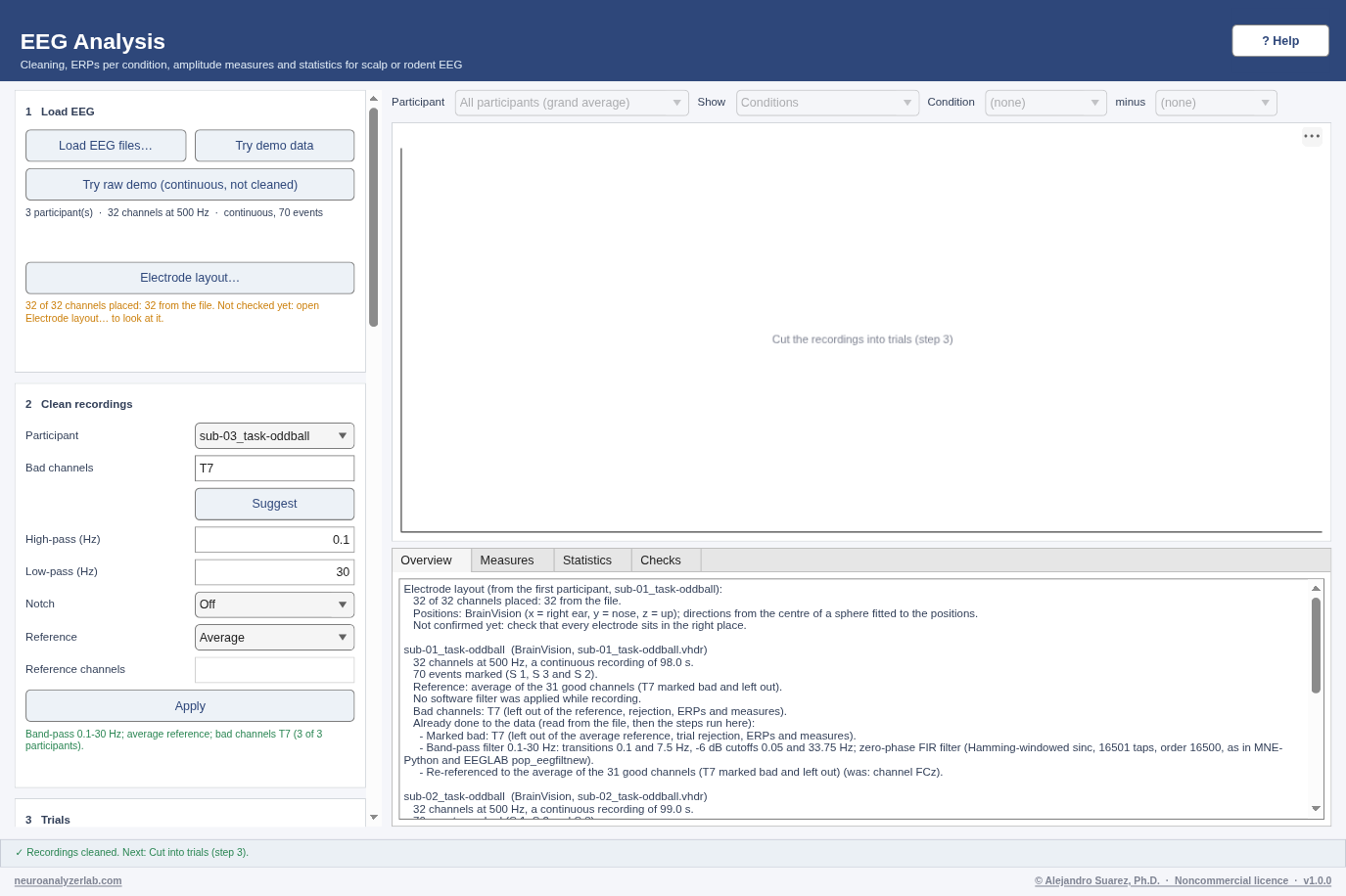
- 1 Load EEG: Load EEG files… (one file per participant: EEGLAB .set, FieldTrip .mat, BrainVision .vhdr, EDF / BDF, XDF, EEG-BIDS or a plain .mat), Try demo data (8 cleaned participants) or Try raw demo (continuous, not cleaned) (3 raw recordings).
- Read the Overview tab: channels, trials per condition, reference, electrode positions and what was already done to the data, then every step done here.
- Electrode layout… (step 1): check the drawing and the Status column, fix the Source, a Positions file… or a name in As if needed, and click Use this layout. Positions are needed only for scalp maps.
- 2 Clean recordings (raw data): Bad channels per participant (or Suggest), High-pass, Low-pass and Notch filters, the Reference, then Apply.
- 3 Trials: Events and names (e.g.
S 1 = Standard, S 2 = Target), Trial from / to (ms), Reject trials by Peak-to-peak and/or Absolute amplitude, then Cut into trials (or Apply rejection for files already cut into trials). The Checks tab lists what was checked in the trials (click a row for why it matters and what to try; Show ERPs and Measure update it). - 4 ERPs: baseline (−200 to 0 ms by default), Channels to plot (e.g.
Pz), Show ERPs; choose the participant or grand average and the view above the plot. - 5 Measure: mean amplitude (recommended) or peak amplitude, the time window and channels, then Measure (Measures tab).
- Scalp maps (step 5, next to Measure): the mean voltage of every electrode in the same window, drawn on the head (or on the skull for rodents), one map per condition and one of A minus B; confirm the electrode layout first. Show → Conditions brings the ERPs back.
- 6 Statistics: Parametric or Nonparametric, Compare conditions (Statistics tab; the Checks tab adds the checks of the test).
- 7 Time–frequency (optional): Frequencies (e.g. 4 to 40 Hz), Wavelet cycles, Baseline, Channels (e.g.
Oz) and Band, then Time–frequency; Show chooses Time–frequency (ERSP), Phase locking (ITPC) or Band power. Grey = no value (the wavelet would reach beyond the trial). - 8 Save: Export results… (.csv or .mat), Save session… (it replays every cleaning step from the files), Report (PDF)…, Methods text….
Electrode layouts, cleaning, checks, scalp maps, time–frequency, demo expectations, inputs, outputs and troubleshooting are on the EEG page.
 DEMO DATA — synthetic, generated by core/demo/demoEEG.m
Response features
Signal Characterization
Turn each response into numbers (latency, onset delay, FWHM, AUC, rise / decay time, amplitude), compare groups of animals statistically and export publication figures. More on this pipeline.
Quick start
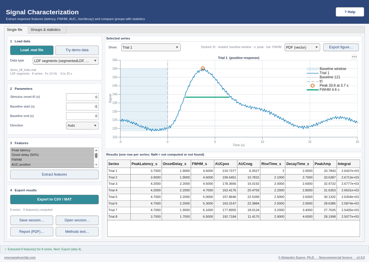
- Load data: click Load .mat file. The data type is detected (LDF segments, ERP / average, time series) and the number of series, Fs and time range are shown; the first series is plotted.
- Parameters: set the stimulus onset t0 (s), the baseline window (s) and the response direction. The plot shows t0 (dashed), the baseline window (shaded) and the detected peak and FWHM, so you can check them before extracting.
- Features: select the features (Ctrl/Cmd-click for several) and click Extract features.
- Export: check the table (click a row to plot that series) and click Export to CSV / MAT. Export figure… above the plot saves the selected trace as a publication figure.
- Groups & statistics tab (or Try group demo): in 1 Files and groups type a Group name and click Add files… (one .mat per animal); repeat for each group. The # column is the subject number: paired designs match #1 with #1, #2 with #2 (fix with ▲ Move up / ▼ Move down).
- Feature and test: choose the Feature, Value per (File (mean trace) recommended: one animal = one file), Onset t0 (s), Baseline (s) and Direction; then the Design (Paired, Unpaired, ANOVA for 2+ independent groups, or Repeated measures when the same animals appear in 3+ conditions), the Method (Parametric or Nonparametric) and, for two groups, Compare A vs B (difference = B − A). Click Run test: the Plot tab shows every animal (with repeated measures, each animal’s line across the conditions), mean ± SEM (or Box plot) and the significance brackets; the Results tab lists test, statistic, df, p, effect size, 95% CI, n, sphericity and its corrections (repeated measures), a robustness check with the other test family, assumptions and a copy-ready report; the Checks tab lists what was checked before you use the result (n, normality, sphericity, equal spread, agreement of the two test families, missing values; click a row for why it matters and what to try).
- Export: choose a format and click Export figure… (PDF / SVG / EPS vector, or PNG / TIFF at 300 or 600 dpi; 8.5 cm wide, 8 pt Helvetica, the window is not changed). Export values & report… saves the per-animal values (.csv plus a _report.txt) or the full result (.mat).
- Session / report (optional): in step 4 of either tab, Save session… stores the single file and every group file (with checksums), all settings and results; Open session… re-extracts the features and re-runs the test; Report (PDF)… writes a one-page summary. See Sessions and reports.
 DEMO DATA — synthetic, generated by core/DemoData.m
Demo data
- Data:
demo_ldf_trials.mat, 8 LDF trials from −5 to 20 s at 10 Hz (0 = stimulus onset). The demo sets t0 = 0, direction Auto, the baseline to −5–0 s and selects every feature. - Expected per trial (true response: ~120 PU baseline + 30 PU gamma-shaped hyperemia): peak latency ≈ 4 s, peak amplitude ≈ 30 PU, onset delay (50%) ≈ 1.9 s, FWHM ≈ 5.5 s, rise time (10–90%) ≈ 2.2 s, decay to 50% ≈ 3.4 s; positive direction.
- Trials differ by a few PU / tenths of a second because of vasomotion and noise, which is why the mean over trials is the number to report.
- Group demo (Try group demo): 24 files,
control_animal01.mat…drug_animal08.mat: the same 8 animals in Control, Stimulated and Drug, each with 8 LDF trials (−5 to 20 s at 10 Hz). True peak hyperemia 18, 30 and 24 PU; animals differ by ~3 PU, plus ~2.5 PU per animal and condition. - Paired t-test, Peak amplitude, Control vs Stimulated: Stimulated − Control ≈ +12 PU (95% CI roughly +9 to +15), p < 0.001, d_z ≈ 3.5 (simulated 3.3). Wilcoxon signed-rank: p ≈ 0.008 (all 8 animals increase; the smallest exact p possible with 8 pairs). Unpaired (Welch): also significant, with a smaller t.
- ANOVA: F(2, 21) large, p < 0.001; Tukey–Kramer Stimulated − Control ≈ +12 PU (p < 0.001); Drug lies ~6 PU from each of the others (usually, not always, significant). Peak latency ≈ 4 s in every group: no difference expected.
- Checks (group demo, any design): no warnings. Sample size OK (8 animals, one value per file), Normality OK (Shapiro–Wilk does not reject it), Robustness check OK (both test families significant). Set Value per to Each series and run again: Sample size becomes a Warning, because the 64 trials per condition come from 8 animals (pseudoreplication).
- Faults study (
groups_faults/in the demo folder: in Files and groups addcontrol_animal01–06.matas Control,stimulated_animal01–06.matas Stimulated anddrug_animal01–06.matas Drug): Repeated measures, Peak amplitude, Run test. The Checks tab gives Sample size a Check (6 animals, fewer than 8), Normality a Check (the residuals are not normal; the most extreme value isstimulated_animal06.mat) and Sphericity a Check (violated: Mauchly's test p < 0.001, Greenhouse–Geisser ε about 0.5, so the corrected p is reported). The test is still significant either way, so the Robustness check is OK. Paired, Control vs Stimulated: Normality a Check (animal 6's difference, about +40 PU against about +12 PU for the others).
Inputs and outputs
In
- LDF trials from LDF Process:
segmentedLDF,segmentedTime(one series per trial); the trials of Save trials… in the Laser speckle window have the same format (% change of one ROI) - LFP from Extract Ephys:
lfp_data,t_lfp(mean over channels = one series) - ERP export from LFP analysis, or any
.matwithtandy(ortandLDF)
Out
- .csv: one row per series, columns Series, PeakLatency_s, OnsetDelay_s, FWHM_s, AUCpos, AUCneg, RiseTime_s, DecayTime_s, PeakAmp, Integral
- .mat:
data(the table as a cell array) andcolNames - Groups & statistics, Export values & report…: .csv with
Group, Subject, <feature>plus<name>_report.txt, or .mat with the structresults(the test, its checks and the settings)
Troubleshooting: 17 common problems
| Problem or message | What to do |
|---|---|
| "… does not contain a supported format" | The file needs segmentedLDF + segmentedTime, lfp_data + t_lfp, or t + y (or t + LDF). The alert lists the variables it found. |
| Series skipped (t and y lengths differ) | Each y must have one value per time point; check the saved variables. |
| Features are NaN | Check t0 (inside the time range?) and the direction; the plot shows where the peak was found. |
| Peak found on the wrong deflection | Set Direction to Positive or Negative instead of Auto. |
| "The paired design needs the same number of subjects in both groups" | Every animal needs one file in each group. Add the missing file or remove the extra one; the # column shows the pairing. |
| Wrong animals paired | The Results report lists every pair (1: fileA ↔ fileB). Files are added in alphabetical order; fix the order with ▲ Move up / ▼ Move down. |
| Run test is disabled | Add files to at least two groups. For a two-group design, choose two different groups in Compare. |
| "… excluded because the feature could not be computed" / "… left out: the feature could not be computed" | The feature was NaN for those files (peak not found or never crossing 50%). Check Onset t0, Baseline and Direction, or choose another feature. |
| Checks: every series counted as a subject | Set Value per to File (mean trace): one value per animal. Trials of one animal are not independent, so counting them as subjects makes p far too small. |
| Checks: not normal | Look at the Plot tab for the animal named in the row. Report the rank-based result (Method: Nonparametric) or both; do not remove an animal only because it is extreme. |
| Checks: the rank-based test cannot reach p < 0.05 | With 5 pairs or fewer (3 vs 3 unpaired) the exact rank test cannot be significant whatever the data. Add animals, or report the parametric result with its normality check. |
| "The parametric and rank-based tests disagree" | Usually few animals or an outlier. Look at the Plot tab, and report the rank-based result or add animals. |
| Same animals in 3 or more conditions | Choose Design: Repeated measures (same animals, 3+ conditions). The one-way ANOVA assumes independent groups and is less powerful here. |
| "Repeated measures need one file per animal in every group" | Every animal needs one file in each condition. The alert lists the files per group; add the missing files or remove the extra ones, and check the # order in the Files tab. |
| "Sphericity: violated" | The variances of the differences between conditions are not equal, so the Greenhouse–Geisser corrected p (non-integer df, e.g. F(1.3, 9.1)) is reported. You can also report the Friedman test (Method: Nonparametric). |
| Export figure… is disabled | Run a test first (Groups & statistics), or load a file (Single file). |
| The journal wants Arial or another size | Export as PDF or SVG (vector) and change the font or size in Illustrator or Inkscape; the text stays editable. |
All pipelines · many files
Batch Processing
Run one analysis with the same settings on a whole folder and get one summary table. More on this pipeline.
Quick start
- Pipeline: choose what to run on every file: LDF: trials + response features, LFP: ERP (+ CSD) per channel, MUA: spike sorting per channel, EEG: ERPs and a measure per condition, Imaging: ROI dF/F and vessel diameter or Response features (any trace file). The line below says which files it reads. Try demo batch adds a few synthetic files with known answers and fills the settings.
- Input files: click Add folder... (every file of the folder that this pipeline reads) or Add files... (multi-select). Select files and click Remove to drop them; Clear empties the list. Files are processed in list order.
- Settings: one set of settings for every file (hover a field for its unit and meaning). They are the settings of the matching window: e.g. downsampling, filter and trial window for LDF; epoch, N1 window and electrode spacing for LFP; detection, clustering and random seed for MUA; bad channels, filters, reference, events, trial window, rejection, baseline and the measure for EEG.
- Run: choose the Output folder... and click Run batch. The table and the status bar show which file is being processed; Cancel stops before the next file. A file that fails does not stop the batch: it gets a red row with the reason.
- Results: one row per file (LFP and MUA: per channel; EEG: per condition; imaging: per ROI). Green = ok, orange = warning (some channels failed), red = error, gray = skipped. Open folder shows the summary (.csv and .mat), the log (.txt) and, for LDF, the trial files; Export... saves a copy of the table (.csv, .xlsx or .mat).
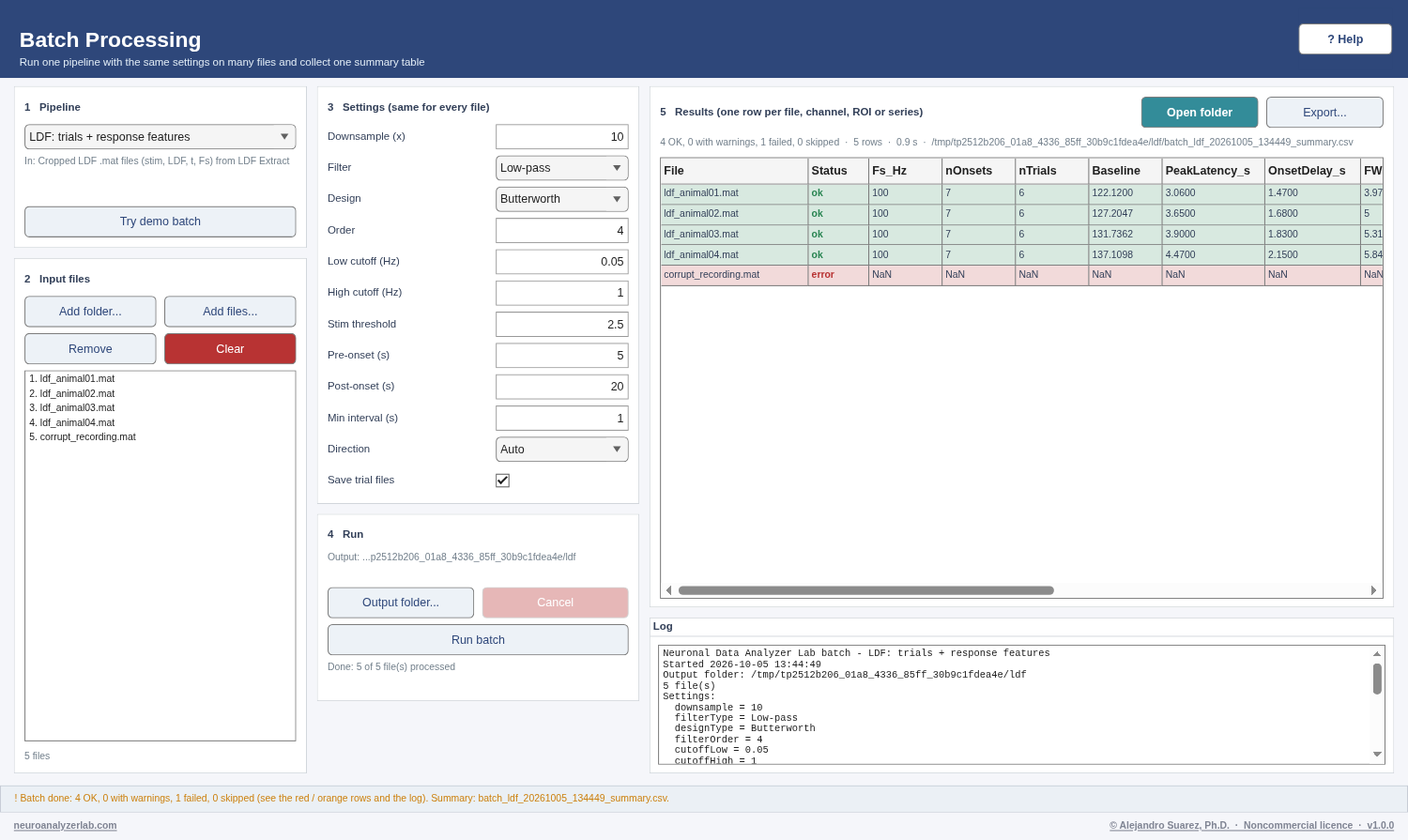 DEMO DATA — synthetic, generated by core/demo/demoBatch.m
Demo data
- Data: Try demo batch writes synthetic files for the chosen pipeline, each with slightly different known answers, and fills the settings.
- LDF: 4 cropped recordings (200 s, 7 stimuli of 5 s). What you should get: 7 onsets and 6 trials per file (the last stimulus is too close to the end); peak latency ~3, 3.5, 4 and 4.5 s and peak amplitude ~20, 25, 30 and 35 PU (within ~2 PU); one trial file per recording in the trials folder. The Checks column of each file says 1 to check: Trials (that left-out stimulus) and nothing else.
- LFP: 3 recordings, 8 channels 100 µm apart. What you should get: 8 rows per file; the N1 is largest and the CSD sink (SinkChannel) is on channel 3, 4 and 5, with the N1 at ~12, 15 and 18 ms (roughly −100 to −140 µV on the sink channel). The Checks column says OK for every file.
- MUA: the demo MUA recording and a copy recorded at twice the gain, channel 4. What you should get: 2–3 units and the same spike count in both files (sorting does not depend on the gain); the evoked rate (5–55 ms after each stimulus) is several times the baseline rate. The Checks column has no warnings; Signal-to-noise may be a Check when a weak cluster (unit 3 seen from channel 5) is kept.
- EEG: the 3 raw recordings of the EEG demo (BrainVision, 500 Hz, 32 channels against FCz, a noisy T7, blinks in 8 trials each); the settings mark T7 bad, filter 0.1–30 Hz, re-reference to the average, cut −200 to 800 ms around S 1 = Standard, S 2 = Target, S 3 = Novel, reject above 100 µV peak-to-peak and measure the mean amplitude 300–400 ms at Pz. What you should get: 3 rows per file (Standard, Target, Novel), 62 trials per file with exactly the 8 blink trials rejected, and the P300 Target (about 5.6 to 7.7 µV) > Novel (about 3.4 to 4.7 µV) > Standard (about 0.7 to 1.9 µV) in every file: the same numbers as EEG Analysis with the same settings. The Checks column has no warnings; Trials per condition is to check (Target and Novel keep fewer than 20 trials, enough for the P300).
- Imaging: 3 stacks with a cell (roiMask) and a vessel crossed by the line 25 50 63 50. What you should get: peak ΔF/F ~0.5, 1.0 and 1.5 at ~6.7 s (the second of two transients, which rides on the tail of the first) and mean vessel diameter ~10, 12 and 14 px.
- Response features: 4 trial files. What you should get: peak latency ~3, 3.5, 4, 4.5 s and peak amplitude ~20, 25, 30, 35 PU (one row per file); Series = Each series gives one row per trial (32 rows).
Inputs and outputs
In
- LDF: cropped
.matfiles from LDF Extract (stim,LDF,t,Fs) - LFP:
.matfiles from Extract Ephys (lfp_data,stim_data,lfp_fs,stim_fs;t_lfp,lfp_channelsandlfp_spacing_umoptional: Spacing 0 uses each file'slfp_spacing_um) - MUA:
.matfiles from Extract Ephys (mua_data,mua_fs;t_mua,mua_channels,stim_data+t_stimoptional) - EEG: one file per participant, raw or cleaned, as EEG Analysis reads it: BrainVision
.vhdr(with its.vmrkand.eeg), EDF / BDF, EEGLAB.set, FieldTrip.mat, XDF (EEG-BIDS: itssub-…_eegfile). Plain.matarrays need the form of EEG Analysis (a red row says so) - Imaging:
.matwithstack(orframes), optionaltimeVec/tandroiMask/roiMasks, or a multi-frame TIFF - Response features: any file Signal Characterization reads (
segmentedLDF+segmentedTime,lfp_data+t_lfp,t+y,t+LDF)
Out
<name>_summary.csvand<name>_summary.mat(tablesummary+ structbatchwith the pipeline, settings, files, statuses, messages, log and date; Export… in the window saves the same two variables): columns File, Status, Message, then the pipeline's results- LDF, LFP, MUA and EEG: a Checks column: the checks of the matching window (LDF Process, LFP Analysis, MUA Analysis, EEG Analysis) in one cell (OK, 1 to check: Topic: … or 2 warnings: Topic: …, the first of the most serious kind): per file for LDF, LFP and EEG (the same on every row of the file), per channel for MUA; the log line of each file ends with the same. The checks do not change the Status: read them before using the numbers
<name>_log.txt: date, settings and one line per file (result or error)- LDF:
trials/<file>_segments.matper recording (segmentedLDF,segmentedTime,Fs), ready for LDF Average
Troubleshooting: 12 common problems
| Problem or message | What to do |
|---|---|
| A row is red with "Missing variable(s)" | The file was not saved by the step this pipeline expects (e.g. a raw LabChart export in the LDF pipeline). Use the files named under Inputs, or choose the matching pipeline. |
| A row is red with "Unable to read" / "not a binary MAT-file" | The file is damaged or not a MAT file. Remove it (select it, Remove) or re-export it; the other files are not affected. |
| LDF: "No stimulus onsets found above threshold" | The stimulus never crosses Stim threshold: lower it (e.g. 0.5 for a 1 V trigger, 2.5 for 5 V TTL). |
| LDF: "no complete trial fits" | Pre-onset + Post-onset is longer than the recording around the stimuli: shorten the windows. |
| LFP: "Channel(s) … not in the file" | The Channels field lists numbers the file does not have: clear it (all channels) or use the numbers shown in LFP Analysis. |
| MUA: a red channel row (file orange) with "Too few spikes for clustering" | That channel has almost no spikes at this threshold: lower Threshold (k) or Min spikes / cluster, or leave the channel out; the other channels of the file are kept. |
| EEG: a red row with "does not make clear which variable holds the EEG" | A plain .mat array does not say which variable is the EEG: open it in EEG Analysis (a short form asks), or save it as an EEGLAB .set or FieldTrip .mat. |
| EEG: a red row with "No good channel to measure at" | Every channel in Channels is marked bad in that file (typed in Bad channels or suggested): choose other channels. |
| EEG: "Every trial exceeds the threshold" / few trials left | One noisy channel can fail every trial: add it to Bad channels (or tick Also suggested bad channels), check the filters (no high-pass leaves drift in), or raise the rejection threshold. |
| Imaging: "needs a line" or no diameter columns | Type the line across the vessel in Line x1 y1 x2 y2 (px) (read the coordinates in ROI Analysis). |
| Imaging: "No ROI" | The stacks have no roiMask: draw and export ROIs in ROI Analysis, or measure Vessel diameter only. |
| The batch takes long | MUA sorting is the slowest part (seconds per channel): select only the channels you need. Cancel stops after the current file and still writes the summary of the files done. |
All windows
Sessions and reports (every window)
Save everything needed to repeat an analysis, reopen it later, and write a one-page PDF report. More on this pipeline.
Quick start
- Save session… (last step card of every analysis window): choose a file name, type optional notes (animal, condition, why these settings) and click Save session. The
.nasession.matfile stores the input file paths with their size, date and MD5 checksum, every setting, the results and your notes. - Open session…: choose a
.nasession.matsaved by the same window. The input files are reloaded and checked; the settings are applied and the analysis is re-run, so the window looks as it did when you saved. - If an input file has moved, put it next to the session file (it is found automatically) or choose it when asked. If a file has changed since the session was saved, the session still opens and the status bar warns you.
- Report (PDF)…: writes one A4 page with a picture of the window and, below it, the Neuronal Data Analyzer Lab and MATLAB versions, the date, every input file with its MD5, the window's checks (warnings first), the settings and the key results. Attach it to your lab notebook or use it for the methods section.
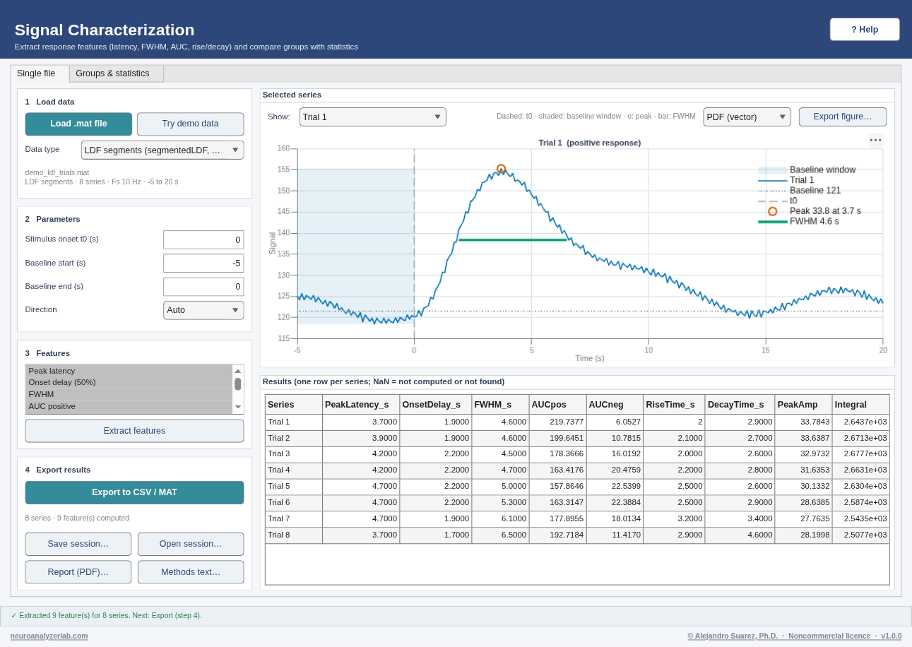 DEMO DATA — synthetic, generated by core/DemoData.m
Demo data
- Try: in any window click Try demo data, run the analysis, then Save session…. Close the window, open it again from the launcher and click Open session…: the same plots and numbers come back.
- What you should get: the status bar says "Session … opened (saved … with Neuronal Data Analyzer Lab v…)" and shows your notes. Report (PDF)… writes a one-page PDF (about 100–200 kB).
Inputs and outputs
In
- A
.nasession.matfile saved by the same window (Open session) - The input files the session refers to, at their saved location, next to the session file, or chosen when asked
Out
<name>.nasession.mat: variablesessionwithformat,formatVersion(1; a file from a newer format is refused with a message to update the toolbox, older ones are upgraded when opened),app,appTitle,toolboxVersion,matlabVersion,os,created(ISO 8601),inputs(role, path, name, bytes, modified, md5),settings,results,summary,checks(level, topic, found, why, action),notes<name>_report.pdf: one A4 page (window image + versions, inputs with MD5, checks, settings, key results)
Troubleshooting: 5 common problems
| Problem or message | What to do |
|---|---|
| "This session was saved by …, not by this window" | Open the session in the window named in the message (each window saves its own kind of session). |
| "Session not opened: … not found at …" | The input file was moved or renamed. Copy it next to the session file, or use Open session… again and locate it when asked. |
| "… has CHANGED since the session was saved (MD5 differs)" | The input file is not the one used when the session was saved (edited, re-exported or overwritten). The results may differ; use the original file if you still have it. |
| Report not written | Check that the folder is writable and that the PDF is not open in another program. The analysis itself is not affected. |
| The window picture in the PDF shows only one plot | exportapp is not available (MATLAB older than R2020b or no display); the largest plot was used instead. |
Getting help
The Help window
Every window's ? Help button opens its topic in the Help window, which has a topic list in workflow order, Previous / Next, and ▶ Try it with demo data, which opens that window with its demo loaded. On the Welcome topic the button writes every demo file to a folder instead and offers to make it the Import folder. Learn more opens the matching page of this website in your browser; the footer of the launcher and of every window also links to it.