Pipeline
Response features, group statistics and figures
Signal Characterization turns each response into numbers, compares groups of animals with statistical tests and exports publication figures.
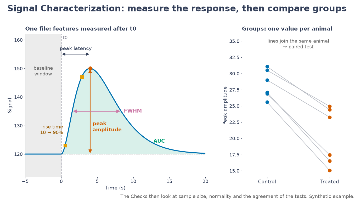
Features of a single response
Reference level and direction
- Baseline: the mean of the signal inside the baseline window is the reference for every feature. If the window holds no samples, the pre-onset mean is used; if end ≤ start, the first 0.05 s of the trace. For trials that start before t0 the window is set to the pre-stimulus part when the file is loaded.
- Direction: Positive (peaks), Negative (troughs) or Auto (negative when the post-onset deflection below baseline is larger than above).
Features (measured after t0)
- Peak latency: time from t0 to the peak.
- Onset delay (50%): time from t0 until the response first reaches 50% of the baseline-to-peak amplitude.
- FWHM: width of the part of the response around the peak that stays beyond half of the baseline-to-peak amplitude.
- AUC positive / negative: area above / below the baseline over the whole trace.
- Rise time: 10% → 90% of the baseline-to-peak amplitude, before the peak.
- Decay time: from the peak until the signal returns past 50%.
- Peak amplitude: peak minus baseline.
- Stim–response integral: integral of the signal from t0 to the end.
A feature that cannot be measured (e.g. the signal never returns to 50%) is NaN.
 Illustration
Data types detected on loading: LDF trials (one series per trial; also the trials saved by the Laser speckle window, in the same format), LFP from Extract Ephys (mean over channels), an ERP export, or any file with t and y. The plot marks t0, the baseline window, the detected peak and the FWHM before you extract, so the settings can be checked.
Groups & statistics
In the Groups & statistics tab, add one .mat file per animal to each group. One value per animal is computed for the chosen feature (recommended: from the file's mean trace), then tested:
| Design | Parametric | Nonparametric (ranks) | Effect size |
|---|---|---|---|
| Paired (same animals, 2 groups) | Paired t-test | Wilcoxon signed-rank[16] | dz; rank-biserial r |
| Unpaired (2 groups) | Welch t-test[14] | Mann–Whitney U[17] | Hedges' g; rank-biserial r |
| ANOVA (2+ independent groups) | One-way ANOVA with Tukey–Kramer comparisons[15] | Kruskal–Wallis[18] | η², ω²; η²H |
| Repeated measures (same animals, 3+ conditions) | Repeated-measures ANOVA with sphericity test[27] and corrections[28][29]; Holm-corrected[30] paired t-tests | Friedman test[31]; Holm-corrected Wilcoxon signed-rank tests | partial and generalized η², dz; Kendall's W |
- Every result lists the test, statistic, df, p, effect size, 95% CI of the difference, n per group, a robustness check with the other test family, the assumptions, and a copy-ready report sentence.
- Paired designs match subject #1 with #1, #2 with #2 (the # column; reorder with Move up / Move down); the report lists every pair.
- The plot shows every animal, pair lines, mean ± SEM or a box plot, and significance brackets.
- Repeated measures: when the same animals are measured in 3 or more conditions, choose Design: Repeated measures. Animal #1 of every group is the same animal, and so on; every group needs the same number of files, and an animal missing a value in any condition is left out of all of them (the assumptions say how many).
- Sphericity: the repeated-measures ANOVA assumes that the differences between every two conditions vary by the same amount. Mauchly's test checks this; when it fails (p < 0.05), the Greenhouse–Geisser corrected p is reported (df with decimals, e.g. F(1.3, 9.1)); all three p-values (uncorrected, Greenhouse–Geisser, Huynh–Feldt) are listed. With few animals Mauchly's test has little power: if the corrected p leads to another conclusion, report the corrected one.
- The Friedman test ranks the conditions within each animal, so it needs neither normality nor sphericity. Kendall's W goes from 0 (no consistent order) to 1 (every animal ranks the conditions the same way).
- With repeated measures the plot draws each animal's line across the conditions. Not available: mixed models (for example missing values kept, or two within-animal factors); use a statistics package for those.
Checks
After every Run test, one row per check (they never change the result): They are in the Checks tab next to Files, Results and Plot; click a row for why it matters and what to try. EEG Analysis runs the same checks after Compare conditions, worded for participants (see EEG).
- Sample size: n per group (animals: one value per file). Warning when Value per is Each series (trials of one animal are not independent: n and p would be wrong, pseudoreplication), when a group has fewer than 3, or when the rank-based test reported cannot give p below 0.05 with these n whatever the data (exact Wilcoxon: 2 / 2ⁿ, e.g. 0.0625 for 5 pairs; Mann–Whitney 3 vs 3: 0.1; a Check when it is only the robustness check). Check below 8 animals: one animal can change the verdict.
- Normality: Shapiro–Wilk test (Royston's algorithm, as in R and SciPy) on what the parametric test assumes normal: the paired differences, the values of each group, or (repeated measures) the residuals, each value minus its animal's and its condition's mean. Check at p < 0.05, Warning when the rank-based test also gives another verdict (report it instead); OK with a rank-based result. The most extreme animal (more than 3.5 robust SDs from the median) is named. With few animals the test misses departures: look at the Plot tab too.
- Sphericity (repeated measures, 3+ conditions, parametric): Check when Mauchly's test rejects it (the Greenhouse–Geisser corrected p is reported) or cannot be computed; Warning when the uncorrected p is reported but the corrected one gives another verdict at 5% (report the corrected one). The Friedman test needs no sphericity.
- Equal spread (one-way ANOVA, parametric): Check when the largest SD is more than twice the smallest, Warning when the group sizes also differ by more than 1.5 times (ANOVA and Tukey's p are then wrong). The Welch t-test needs no equal SDs.
- Robustness check: a Check when the parametric and the rank-based tests disagree at 5%. Missing values: a Check when animals were left out because the feature could not be computed.
- Checks (group demo, any design): no warnings. Sample size OK (8 animals, one value per file), Normality OK (Shapiro–Wilk does not reject it), Robustness check OK (both test families significant). Set Value per to Each series and run again: Sample size becomes a Warning, because the 64 trials per condition come from 8 animals (pseudoreplication).
- Faults study (
groups_faults/in the demo folder: in Files and groups addcontrol_animal01–06.matas Control,stimulated_animal01–06.matas Stimulated anddrug_animal01–06.matas Drug): Repeated measures, Peak amplitude, Run test. The Checks tab gives Sample size a Check (6 animals, fewer than 8), Normality a Check (the residuals are not normal; the most extreme value isstimulated_animal06.mat) and Sphericity a Check (violated: Mauchly's test p < 0.001, Greenhouse–Geisser ε about 0.5, so the corrected p is reported). The test is still significant either way, so the Robustness check is OK. Paired, Control vs Stimulated: Normality a Check (animal 6's difference, about +40 PU against about +12 PU for the others).
The implementation is checked against published textbook data sets; see Validation. The Shapiro–Wilk test gives the same W and p as SciPy (scipy.stats.shapiro, Roystons algorithm).
Figure export
Export figure… saves the selected trace (Single file tab) or the group plot as a publication figure: vector PDF, SVG or EPS, or PNG / TIFF at 300 or 600 dpi; 8.5 cm wide, 8 pt Helvetica, white background. The window itself is not changed. Vector files stay editable in Illustrator or Inkscape. Plot colours across the toolbox use the colour-blind-safe Okabe–Ito palette[20].
Walkthrough
Walkthrough: repeated measures on the group demo
Inputs and outputs
In
- LDF trials from LDF Process:
segmentedLDF,segmentedTime(one series per trial); the trials of Save trials… in the Laser speckle window have the same format (% change of one ROI) - LFP from Extract Ephys:
lfp_data,t_lfp(mean over channels = one series) - ERP export from LFP analysis, or any
.matwithtandy(ortandLDF)
Out
- .csv: one row per series, columns Series, PeakLatency_s, OnsetDelay_s, FWHM_s, AUCpos, AUCneg, RiseTime_s, DecayTime_s, PeakAmp, Integral
- .mat:
data(the table as a cell array) andcolNames - Groups & statistics, Export values & report…: .csv with
Group, Subject, <feature>plus<name>_report.txt, or .mat with the structresults(the test, its checks and the settings)
Demo expectations
The trials file and the group demo are described on the demo data page. Expected results (from the in-app Help):
- Data:
demo_ldf_trials.mat, 8 LDF trials from −5 to 20 s at 10 Hz (0 = stimulus onset). The demo sets t0 = 0, direction Auto, the baseline to −5–0 s and selects every feature. - Expected per trial (true response: ~120 PU baseline + 30 PU gamma-shaped hyperemia): peak latency ≈ 4 s, peak amplitude ≈ 30 PU, onset delay (50%) ≈ 1.9 s, FWHM ≈ 5.5 s, rise time (10–90%) ≈ 2.2 s, decay to 50% ≈ 3.4 s; positive direction.
- Trials differ by a few PU / tenths of a second because of vasomotion and noise, which is why the mean over trials is the number to report.
- Group demo (Try group demo): 24 files,
control_animal01.mat…drug_animal08.mat: the same 8 animals in Control, Stimulated and Drug, each with 8 LDF trials (−5 to 20 s at 10 Hz). True peak hyperemia 18, 30 and 24 PU; animals differ by ~3 PU, plus ~2.5 PU per animal and condition. - Paired t-test, Peak amplitude, Control vs Stimulated: Stimulated − Control ≈ +12 PU (95% CI roughly +9 to +15), p < 0.001, d_z ≈ 3.5 (simulated 3.3). Wilcoxon signed-rank: p ≈ 0.008 (all 8 animals increase; the smallest exact p possible with 8 pairs). Unpaired (Welch): also significant, with a smaller t.
- ANOVA: F(2, 21) large, p < 0.001; Tukey–Kramer Stimulated − Control ≈ +12 PU (p < 0.001); Drug lies ~6 PU from each of the others (usually, not always, significant). Peak latency ≈ 4 s in every group: no difference expected.
- Repeated measures, Peak amplitude, all three conditions (the same 8 animals, matched by #): repeated-measures ANOVA F(2, 14) large, p < 0.001, partial η² large. Mauchly's test is usually not significant (the demo is simulated with sphericity), so the uncorrected p is reported; Greenhouse–Geisser and Huynh–Feldt p are also < 0.001. Holm-corrected paired t-tests: Stimulated − Control ≈ +12 PU (p < 0.01, d_z ≈ 3.5), Drug − Control ≈ +6 PU, Drug − Stimulated ≈ −6 PU (usually, not always, significant). Friedman: significant (χ²(2) = 14.2, p = 0.0008, Kendall's W = 0.89: almost every animal ranks the conditions the same way).
Step-by-step instructions and troubleshooting: Signal Characterization in the guide.