Pipeline
Laser Doppler flowmetry (LDF) and laser speckle flowmetry
Three windows turn a blood-flow recording (LabChart, AcqKnowledge export, Spike2, EDF or a table) into stimulus-locked trials and a grand average. Signal Characterization then measures each response. Laser speckle images have their own window: Laser speckle flowmetry.
What it does
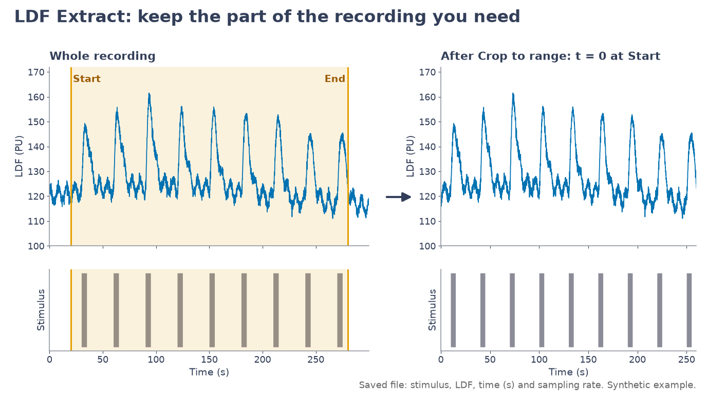
Loads a recording from LabChart, AcqKnowledge exports, Spike2, EDF / BDF or a delimited table. The LDF, Stimulus and Block are guessed from the channel names (the stimulus can also be the comments / event markers of the file, or none). Shows both, and crops the experiment by typing a range or clicking twice on the plot.
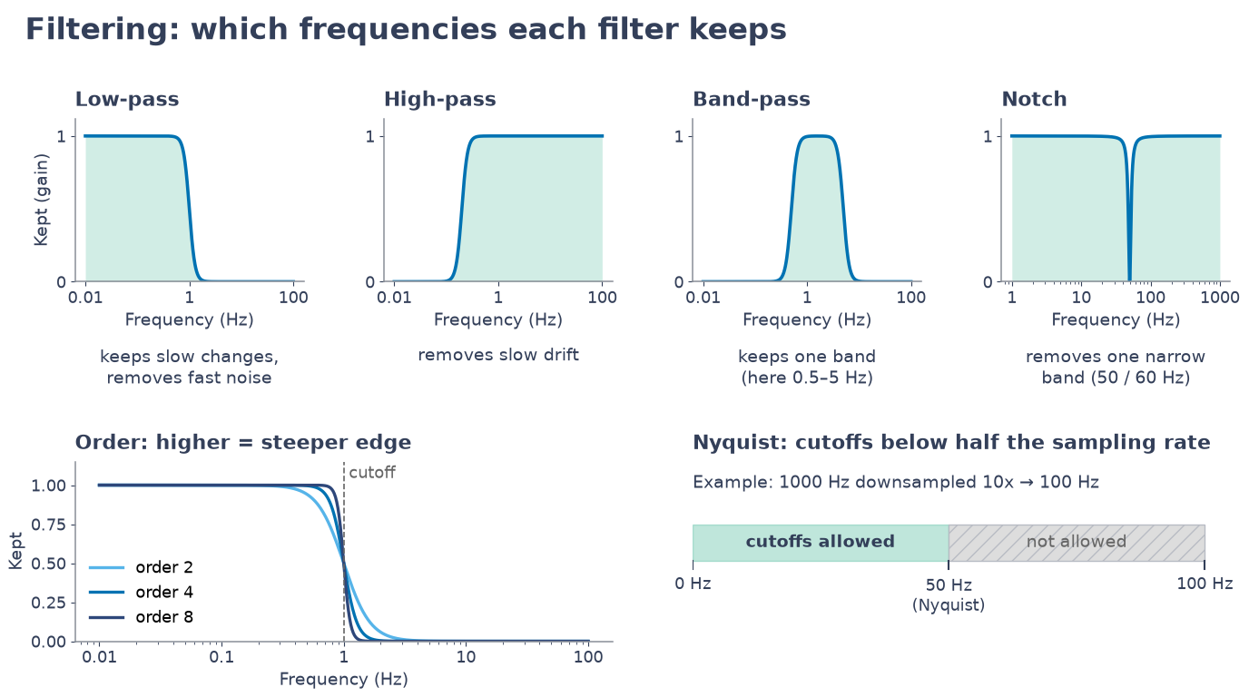
Optional downsampling (1×, 2×, 5×, 10×, anti-aliased) and filtering (low-, high-, band-pass or notch; Butterworth, Chebyshev I or FIR), then trials cut around each stimulus onset. Trials can be appended to an existing trials file.
Pools the trials of one or more trial files (from LDF Processing, or saved by the Laser speckle window) with the same time axis and plots all trials and the grand average (mean ± SD), optionally relative to each trial's pre-stimulus mean.
The LDF channel is used as exported (for example in perfusion units, PU). Laser Doppler flowmetry measures the Doppler shift of light scattered by moving red blood cells[11]; the toolbox does not convert it to absolute flow.
Walkthrough on the demo recording
Inputs and outputs
Extract LDF
In
- LabChart (ADInstruments): MATLAB export
.mat(data,datastart,dataend,samplerate,titles,unittext, comments; every block) or text export (.txt) - AcqKnowledge (BIOPAC): its MATLAB export
.mat(data,isi,labels,units) or its text export. Files saved in AcqKnowledge's own format are not read: save the recording as a MATLAB.mator a text file in AcqKnowledge first - Spike2 (CED): MATLAB export
.mat(one struct per channel withtitle,interval,values; event channels withtimes) - EDF / EDF+ / BDF (
.edf,.bdf; LabChart, clinical and many other systems export it): the channels in their physical units; EDF+ annotations can be the stimulus - Tables (
.txt,.csv,.tsv; PeriSoft, moorVMS-PC, spreadsheets): a header row with the channel names (and optionally a units row), a time column in s, ms or clock time; comma, semicolon or tab separated, decimal point or comma. Without a time column the window asks for the sampling rate. - A cropped LDF
.mat(stim,LDF,t,Fs) opens as well - The flow channel is found by its name or units (LDF, flux, perfusion, flow, PU, BPU); the stimulus by its name (stim, trigger, TTL, pulse…) or because it only has two levels. A LabChart file with 8 or more unnamed channels keeps the old convention: stimulus = channel 6, LDF = channel 8.
Out
- Cropped
.matwithstim(stimulus),LDF(flow),t(time in s, 0 at the crop start) andFs(Hz), and the namesflowName,flowUnits,stimName
LDF Processing
In
.matfrom LDF Extract withstim,LDF,t,Fs(all four are required)
Out
.matwithsegmentedLDF(trials × samples),segmentedTime(s, 0 = stimulus onset, negative = before) andFs
Average LDF Viewer
In
- One or more
.matfiles withsegmentedLDFandsegmentedTime(from LDF Process, or Save trials… in the Laser speckle window)
Out
- Plots of all trials and of the grand average (mean ± SD); the file list shows how many trials came from each file
Variable-level details are on the file formats page.
Methods
Channels and stimulus
The chosen LDF channel sets the time base. A stimulus channel recorded faster is reduced to the LDF rate by taking the maximum over each LDF sample (short pulses are kept); a slower one is held. When the comments / event markers are the stimulus, each one becomes a pulse of height 1 lasting 0.5 s, so LDF Processing finds it with a threshold of 0.5; choose one comment text to use only those comments. The plots are titled with the channel names, and the methods text names the acquisition software and the channels.
Cropping
Sample k is at time (k − 1) / Fs. Cropping keeps samples round(Start·Fs)+1 to round(End·Fs)+1, with 0 ≤ Start < End ≤ duration. Loading a new file, or choosing other channels, discards the previous crop, so a stale crop can never be saved by mistake.
Filtering and downsampling
Downsampling decimates the LDF with an anti-aliasing filter and subsamples the stimulus. Filters are applied forwards and backwards (zero-phase), so responses are not shifted in time. Butterworth filters have a maximally flat pass-band[19]; Chebyshev I filters are steeper with pass-band ripple; FIR filters are always stable but need a high order for a sharp cutoff. Cutoffs must lie below half the sampling rate after downsampling (1000 Hz / 10 → cutoffs below 50 Hz). Processing always starts from the loaded data, so new settings never filter an already filtered signal.
Trials
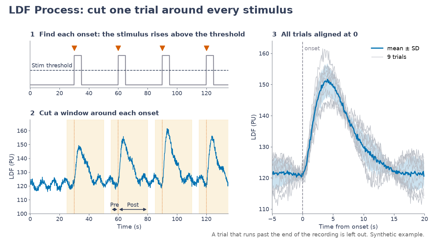
Onsets are the samples where the stimulus rises above the threshold; a crossing closer than the minimum interval to the last accepted onset is ignored, so a train of pulses gives one onset. Each trial runs from onset − pre to onset + post; trials that would run past the start or end of the recording are skipped. Files are pooled in the Average LDF Viewer only when their time axes are identical. Relative to baseline subtracts the mean of each trial's samples before t = 0.
Checks
After Segment trials, one row per check (the same checks run in Batch processing and, for the shared ones, on laser speckle and perfusion images):
- Trials: stimuli left out because their trial does not fit; fewer than 3 trials. Trial baseline: shorter than 2 s or 5 samples.
- Time resolution: one value every dt s after downsampling: Check above 0.5 s (latency and rise time known to within dt), Warning above 2 s.
- Baseline: the mean before the stimuli, usually 30–600 PU for a probe on tissue; outside that a Check (a large vessel under the probe, no contact or bone, or a channel not in PU), never a Warning, because tissue and devices differ.
- Filter: a low-pass below 0.5 Hz smooths the 1–2 s rise (Check); a high-pass above 0.02 Hz shrinks a response lasting several seconds (Check; above 0.1 Hz Warning).
- Baseline drift: a linear fit, in % of the baseline per minute, over the part before the first stimulus when it lasts 60 s or more, else over the trial baselines (4 or more trials over 120 s or more): Check above 3%/min, Warning above 10%/min; a Note when the recording is too short to tell.
- Movement artefacts (on the loaded trace, before filtering): jumps away from the 1 s moving median by more than 8 robust SDs and 25% of the baseline, with their times; Warning when they fall in a trial, Check otherwise.
- Signal range: more than 0.1% of the samples at 0 or below (probe lifted) or stuck at the top (device or export range saturated): Warning.
 Illustration
 Illustration
 Illustration
 Illustration
Demo expectations
These are the results the demo recording should give (from the in-app Help). The recording itself is described on the demo data page.
Extract LDF
- Data: LabChart-style export, 8 channels, 300 s at 1000 Hz. Channel 6 = stimulus: 9 pulses of 5 s every 30 s from t = 30 s. Channel 8 = LDF: ~120 PU baseline with slow drift, vasomotion (0.13 Hz), a cardiac ripple (6 Hz) and noise.
- What you should see: after each stimulus pulse the LDF rises by about +30 PU, peaking about 4 s after the onset, and returns to baseline within ~12 s.
- Try: crop 20 to 280 s (this is exactly what the LDF Process demo file contains) and save; the cropped plots start at t = 0 with the first pulse at 10 s.
- Other formats:
core/demo/demoLDFFormats.mwrites the same recording at 100 Hz as a LabChart text export, a PeriSoft-style table, a Spike2 export, a table without a time column (type 100 Hz when asked) and an EDF+ file, so each one can be opened in Extract LDF and checked against the same answer.
LDF Processing and filtering
- Data: the cropped demo recording (20–280 s of the LDF export, 1000 Hz): 9 stimulus pulses of 5 s, the first at 10 s, then every 30 s.
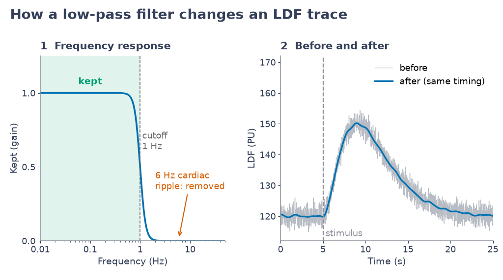
- Try: downsample 10x, low-pass ~1 Hz (removes the 6 Hz cardiac ripple), then segment with pre = 5 s and post = 20 s.
- What you should get: 8 complete trials (the last pulse is too close to the end for a 20 s window). The mean response rises after 0 s and peaks ~4 s after onset at ~+30 PU above a ~120 PU baseline.
- Checks: no warnings; one Check, Trials (1 of 9 stimuli left out: its trial does not fit); OK for the baseline (~120 PU), drift (about −1.4%/min from the 8 trial baselines), movement artefacts, signal range, the filter and the time resolution.
- Faults demo: load
demo_ldf_faults.matfrom the demo folder and segment with the same settings: Baseline drift is a Check (about +5.4%/min), Movement artefacts a Warning (jumps at 31 and 72 s, the second in trial 3) and Signal range a Warning (0.38% of the samples at 0).
- Data: the cropped demo LDF (1000 Hz). Besides the ~+30 PU responses it contains a slow drift (period 400 s), vasomotion at 0.13 Hz (±3 PU), a cardiac ripple at 6 Hz (±1.5 PU) and white noise.
- Low-pass 1 Hz (after 10x downsampling): the 6 Hz ripple and most noise disappear, the responses keep their shape and timing (zero-phase filtering: the peak stays ~4 s after onset).
- High-pass 0.2 Hz: removes drift and vasomotion but also shrinks and distorts the slow (~5 s wide) responses, a good example of a cutoff that is too high for LDF.
Average LDF Viewer
- Data:
demo_ldf_trials.mat, 8 trials from −5 to 20 s at 10 Hz (0 = stimulus onset). - What you should get: the grand average is flat before 0 s (at 0: the demo ticks Relative to baseline; untick it to see the ~122 PU baseline), rises after onset and peaks ~4 s after onset at ~+30 PU, then returns to baseline by ~12–15 s. The SD band shows the trial-to-trial vasomotion (a few PU).
- With Relative to baseline the curve starts at ~0 PU and peaks at ~+30 PU.
Step-by-step instructions and troubleshooting: Extract LDF, LDF Processing, Filtering, Average LDF Viewer.
Laser speckle flowmetry
The Laser Speckle Flowmetry window (launcher → Blood flow → Laser speckle) maps blood flow from laser speckle images: the speckle contrast in every pixel, a flow index, the flow in regions over time, the response to each stimulus and where the flow changed. It opens raw speckle images from the camera, speckle contrast images, or the perfusion / flux images a commercial system exports (.mat, multi-frame TIFF or video; the type is judged from the images when the file does not say).
- Load images: click Load images… and choose a .mat (frames H × W × N), a multi-frame TIFF or a video (or Try demo data). Check Images are: Raw speckle images straight from the camera, Speckle contrast (K) images, or Perfusion / flux images already computed by a commercial system (used as they are). Check the Frame rate and, for the 1/τc model, the Exposure (read from the file when it says).
- Contrast and flow (raw images): Spatial contrast in a 7 × 7 window is the usual choice; Frames per value averages the contrast of several frames (set to about 2 values per second when you load). Type the camera Dark level (an image with the laser off). Flow index: 1/K² (the speckle flow index), or 1/τc from the exposure model.
- ROIs: click Add ROI and drag a rectangle over each region (the ROIs of a .mat file are loaded with it). Without ROIs the whole image is one region.
- Stimulus, trials and Run: Onsets from the stimulus trace in the file, a Regular protocol (first onset, interval, count) or None. Before / After set the trial (the part before 0 s is its baseline) and Resp. from / to the response window. Click Run.
- Read the results: Show → Response map (%) colours where the flow rose (orange) or fell (blue); Average response has one curve per ROI (mean ± SD) with its mean change in the response window in the legend; Flow over time the whole recording; Checks lists what to look at before using the numbers (click a row to read why it matters and what to try).
- Export: Export results… writes a .csv (time, flow change % and flow index per ROI) or a .mat (maps, traces, trials, masks, settings); Save trials… writes the trials of the selected ROI in the LDF trial format, which the Average LDF Viewer and Response features open. Save session…, Report (PDF)… and Methods text… keep the analysis.
Methods
Speckle contrast
A surface lit by a laser shows a grainy speckle pattern. Moving red blood cells change it during the camera exposure, so the pattern is blurred: its contrast K = σ / mean of the intensity drops where blood flows faster (K near 1: still; near 0: fast flow).
- Spatial: K of the pixels in a window around each pixel (5 × 5 or 7 × 7), in every frame[32, 33]. It keeps the time resolution but blurs the image by the window: small vessels look wider, and a region only gives its own contrast where the window stays inside it.
- Temporal: K of each pixel over N frames (15–25 usual)[35]. The image stays sharp; the time resolution drops by N. Needs a still preparation.
- Frames per value (spatial): the K² of this many frames is averaged. Speckle is noisy; averaging frames is standard (commercial systems do it too).
- Dark level: the camera offset adds to the mean but not to the σ, so without subtracting it the contrast is too low.
Flow index
- 1/K² (speckle flow index): for exposures much longer than the decorrelation time τc, K² ≈ β τc / (2T), so 1/K² is proportional to 1/τc and to the speed of the red blood cells[33]. Relative changes of 1/K² follow changes in flow closely; for a +25% flow change it shows about +24%.
- 1/τc (exposure model): solves K² = β (e−2x − 1 + 2x) / (2x²), x = T/τc, for every value[34, 33] and gives 1/τc in 1/s. It needs the exposure T; β (0–1) is the contrast of still speckle for your optics: it changes absolute values, not relative changes.
- Perfusion / flux images from a commercial system are used as they are (their own units).
ROIs, trials and the response map
- The K² (or perfusion) of a ROI's pixels is averaged in each frame, then converted to the flow index. Flow over time is relative to the baseline window (from the start to the first stimulus).
- Each trial is cut from Before to After the onset and expressed as % change from its own mean before 0 s. Average response is the mean ± SD over trials; the response is its mean in the response window (robust); the peak is its largest value after onset (noise makes it larger).
- Response map: in every pixel, the flow of the response window divided by the flow before the onsets (both averaged over trials), minus 1, in %.
Checks
One row per check (Result, Topic, Finding; click a row for why it matters and what to try).
- Raw images: Saturation (saturated pixels lower the contrast), Dark level (none subtracted, or pixels below it), Contrast window (smaller than 5 × 5), Speckle contrast (outside the usual range: static tissue, wrong exposure or already processed images; values above 1), Speckle size (width of the spatial autocorrelation of raw frames: below 1.5 px a Check, since below about 2 px per speckle each pixel averages several and K drops), Illumination (the mean raw intensity changes by more than 10%: laser or light path drift).
- Raw and contrast images: Exposure outside 1–20 ms (Check); Baseline contrast above K = 0.4 in a ROI (Check: static scattering through skull, dura or scar makes 1/K² underestimate relative changes; a thinned skull, a window or multi-exposure speckle imaging help); a Note on the flow index used.
- Perfusion images: Export range (more than 0.1% of the values at the top, e.g. 3000 PU: Warning), and Notes: values are in the device's units (compare relative changes only with the same device and settings), and the dark level and speckle checks need the raw images.
- Every input: Field shift between frames (blocks of frames registered against the first; Check above 1 px, Warning above 3 px), then the blood-flow checks shared with the needle probe, on the ROI traces: Trials, Trial baseline, Time resolution (one value every dt s: Check above 0.5 s, Warning above 2 s or with fewer than 2 values in the response window), Baseline drift, Movement artefacts and Signal range (see LDF Process for the rules). With several ROIs each check is one row, the worst ROI sets its result and the text names the ROIs.
OK is green, Check amber, Warning red, Note grey; the same tab is in every window that has checks.
Inputs and outputs
In
.matwith the images inframesorstack(H × W × N; any numeric type); optionalt(s per frame) orfps,exposureMs,dark(counts),stim(one value per frame, or a faster trace over the same time),roiMasks(H × W × K logical) withroiNames, andkind('raw speckle', 'contrast' or 'perfusion')- Multi-frame TIFF (raw camera frames or exported perfusion / flux images; the frame interval is read from ImageJ TIFFs) or a video (.avi, .mp4: frame rate from the file; avoid compressed videos for raw speckle)
- Perfusion images from commercial imaging systems (their own files are not read): export them as TIFF, video or MATLAB from the system's software and choose Perfusion / flux images
Out
- .csv:
Time_s, then per ROIFlowChange_pct_<ROI>(change from the baseline window) andFlowIndex_<ROI> - .mat: struct
resultswith the maps (flowMean,K2Mean,responseMap),t,roiFlow,roiRel,trials(ROI × trial × sample, %),trialMean/trialSD,response,peak,peakTime,onsets,checks(lines) andcheckRows(the Checks tab rows), the ROI masks and names and every setting - Save trials:
segmentedLDF(trials × samples, % change of the selected ROI),segmentedTime(s from onset),Fs,onsetTimes,roiName,units: the LDF trial format, for the Average LDF Viewer and Response features - Session, one-page PDF report and a draft methods text (see Sessions and reports)
Demo expectations
The demo recording is made by core/demo/demoLSCI.m and described on the demo data page. Expected results (from the in-app Help):
- Data:
demo_lsci.mat(or Try demo data): raw speckle images of a rodent cortex, 80 × 64 px (width × height), 900 frames at 10 Hz (90 s), exposure 5 ms, camera dark level 100 counts (uint16). Each pixel is an independent speckle whose contrast follows the exposure model with β = 1. - Tissue: cortex (parenchyma) with τc = T/20 (K = 0.22), a vessel (x = 14–25 px) with τc = T/200 (K = 0.07, much faster flow) and a static corner (bone, K = 0.70, no flow).
- Stimuli: 5 s pulses at 10, 30, 50 and 70 s (
stimin the file). In an activated disk (centre x = 52, y = 28, radius 12 px) the flow rises by 25% at 4 s after each onset and returns within about 12 s; nowhere else does the flow change. - ROIs in the file: Activated area (inside the disk), Control cortex, Vessel.
- Run with the defaults (spatial 7 × 7, 5 frames per value = 2 Hz, dark level 100, 1/K²): 4 trials; Activated area about +21% in the 2–6 s window (the true mean flow change there is +21.9%; 1/K² sees +21.3%), peak about +28% near 4 s; Control cortex and Vessel about 0% (within ±3%). The response map shows an orange disk of about +20% at the activated area and 0 elsewhere.
- Show → Speckle contrast K: cortex 0.22, vessel 0.07 (light), static corner 0.70 (black). The vessel's edges look wider than 12 px because the 7 × 7 window mixes vessel and cortex there.
- Flow index → 1/τc (exposure model): about 4000 /s in the cortex and 40000 /s in the vessel; the activated area rises slightly more than with 1/K² (closer to the true flow change).
- Dark level 0 instead of 100: the contrast drops by about 5% everywhere and Checks has a Check row, Dark level, asking you to measure it; the relative responses hardly change.
- Checks with the defaults: no warnings. One Check, Speckle size (about 1 px): the demo makes each pixel an independent speckle, which a real camera should not do (2 px or more per speckle). Field shift, exposure, illumination, baseline contrast (K = 0.07–0.22), trials, trial baseline (10 samples), time resolution (2 Hz), movement artefacts and signal range are OK; Baseline drift is a Note: 10 s before the first stimulus and 4 trials over 60 s are too short to judge it.
- Faults demo (
demo_lsci_faults.matin the demo folder): Field shift is a Warning (the image moves by up to 4 px, first above 1 px at 46 s); Illumination (−22%), Exposure (25 ms), Baseline contrast (Thinned skull, K = 0.49) and Speckle size are Checks; the contrast is lower everywhere (two speckles per pixel: cortex K = 0.16). - Perfusion demo (
demo_perfusion_faults.mat, opens as perfusion images): Export range is a Warning (13% of the values at 3000 PU: the vessel), Time resolution a Check (one image per second), and three Notes, among them device units and that the dark level, saturation and speckle size checks need raw images. The activated area still rises by about +20%.
Troubleshooting: 8 common problems
| Problem or message | What to do |
|---|---|
| The contrast is close to 0 everywhere, or flow index values are huge | The images are probably already processed (perfusion or contrast): set Images are accordingly. |
| The contrast is above 0.6 everywhere | Mostly static tissue, a very short exposure, or speckles much larger than a pixel (close the aperture less / zoom out). Check the focus and the laser. |
| The traces are very noisy | Increase Frames per value (e.g. to one flow value per second), use larger ROIs, or record more stimuli. |
| "Type the frame rate" | The file does not say it: type the Frame rate (Hz) in step 1. |
| Stimuli left out (Checks tab) | Their trial (Before … After) does not fit in the recording; shorten Before / After. |
| Field shift (Checks tab) | The head or the camera moved. Register the frames first (ROI analysis, motion correction) or analyse the part before the shift; fix the head and the camera for the next recording. |
| The response is smaller than expected | With spatial contrast, keep ROIs at least half a window inside the activated area: windows that reach outside mix in unchanged tissue. Try 1/τc with the exposure for large changes. |
| "drawrectangle needs the Image Processing Toolbox" | Save the ROIs as roiMasks (H × W × K) in the .mat with the images. |
Walkthrough on the demo stack
Step-by-step instructions: Laser speckle in the guide.