Pipeline
Electrophysiology: LFP and MUA
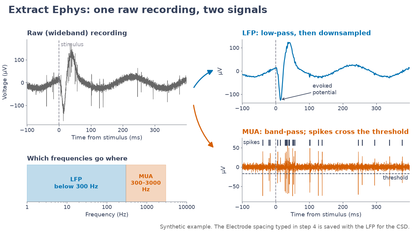
Extract Ephys reads a recording and saves an LFP file and a MUA file. LFP Analysis computes evoked potentials, current source density and time–frequency measures; MUA Analysis detects and sorts spikes.
Extract Ephys
Choose the Source (TDT tank, Intan .rhd or .rhs, Open Ephys binary or legacy folder, NWB, SpikeGLX, Blackrock or Neuralynx; the format is also recognized from the file's extension, folder contents or first bytes), load the recording, pick the stimulus channel and the raw channels, then process:
- Process LFP: optional downsampling by an integer factor after an anti-aliasing low-pass, then an optional 4th-order Butterworth low-pass and an optional 60 Hz notch (zero-phase). The saved rate is the actual one: 24414.0625 Hz / 24 = 1017.25 Hz for TDT data, not the requested 1000 Hz.
- Process MUA: zero-phase band-pass (preset 300–3000 Hz, Butterworth, order 4, or custom). The saved signal is the band-passed trace used for detection.
- Export NWB… writes the processed LFP and its stimulus as an NWB 2.x file (see NWB export).
The channels saved are the ones used when Process was clicked, even if the selection changed afterwards. The methods text names the recording format.
 Illustration
Inputs and outputs
In
- TDT tank / block folder containing the
Whis(stimulus) andxRAW(raw neural) streams (needs the TDT MATLAB SDK,TDTbin2mat, underUtilities/TDTMatlabSDK/) - Intan RHD2000
.rhdfile (file format 1.0–3.x, traditional single-file format) - Open Ephys binary recording folder (GUI 0.5 or later:
structure.oebin,continuous.dat, TTL events) - NWB 2.x
.nwbfile with an ElectricalSeries in /acquisition or /processing - SpikeGLX
.bin+.meta(Neuropixels 1.0 / 2.0 imec AP or LF, nidq) - Blackrock
.ns1–.ns6(NSx 2.1–3.0), with the.nevof the same name for the digital input - Neuralynx folder of
.ncschannels, withEvents.nevfor TTLs - Intan RHS2000
.rhs(stimulation / recording controller, traditional single-file format) - Open Ephys legacy folder:
<processor>_CH<n>.continuousfiles (GUI before 0.6),all_channels.events - Other systems: export the recording from the acquisition software to one of these formats (for example NWB)
Out
- LFP
.mat:lfp_data(channels × samples),lfp_channels,lfp_fs,t_lfp,stim_data,stim_fs,t_stim, andlfp_spacing_umwhen Electrode spacing (µm) is filled in - MUA
.mat:mua_data,mua_channels,mua_fs,t_mua,stim_data,stim_fs,t_stim,filterParams - NWB
.nwb(Export NWB…): LFP in volts in /processing/ecephys/LFP, the stimulus in /stimulus/presentation, electrodes with source channel names. Written with matnwb when installed, otherwise an NWB-style export (not validated).
LFP Analysis
Evoked potentials (ERP)
Stimulus onsets are upward crossings of a threshold by the mean-subtracted stimulus; a crossing closer than the minimum interval to the last accepted onset is dropped, so a train of pulses gives one onset. Each epoch runs from onset − pre to onset + post. Epochs that would run past the recording edges are excluded, not zero-filled, and the ERP is the mean and SD of the valid epochs.
Current source density (CSD)
The CSD is the negative second spatial derivative of the ERP across the ordered channels, divided by the squared spacing[1, 2]. The first and last rows are copied from their neighbours.
Sinks (current flowing into cells) and sources appear with opposite signs across depth. It assumes a linear probe, equal spacing and the true channel order (top to bottom), and at least 3 channels. This is the Standard method, in V/m² (no conductivity).
Spacing (µm) is filled in from the file when it gives lfp_spacing_um; otherwise type your probe's contact spacing (the default is 100 µm).
Step 4 of LFP Analysis has a Method menu with four more estimates. They model the active tissue as discs of a given Diameter (500 µm by default) in tissue of conductivity σ (0.3 S/m for cortex) and give the CSD in A/m³:
- iCSD (inverse CSD[25]) inverts the exact potential of those discs. delta: thin discs at each contact. step: the CSD is constant within half a spacing of each contact. spline: a smooth curve between the contacts. Inverse methods amplify noise, so an optional Smoothing (µm) filters across depth afterwards.
- kCSD (kernel CSD[26]) fits many smooth basis sources of width R with a regularisation λ. When R or λ is 0, both are chosen by cross-validation: each contact is predicted from the others and the best combination is kept. The CSD is also given on a 4× finer depth grid.
- Which method? Standard is fine for a quick look at wide, uniform activity. iCSD is more accurate when the active region is small compared with the probe, and at the top and bottom contacts. kCSD is the most robust to noise and to activity beyond the ends of the probe.
- Only the fields of the chosen method are shown; the plot title names the method (for kCSD also the chosen R and λ). Exports, sessions and the methods text keep the method and its parameters.
On a synthetic laminar recording with a known CSD (core/demo/demoCSD.m, no noise), the relative error is about 0.34 for Standard, 0.10 for iCSD delta, 0.04 for iCSD step, 0.004 for iCSD spline and 0.03 for kCSD; with 1% noise, 0.42 for Standard and 0.11 for kCSD. See Validation.
Time–frequency
- Spectrum: Welch's method[13], 2 s Hann segments with 50% overlap, each segment's mean removed; density in units²/Hz, so the area under the spectrum equals the signal variance.
- Spectrogram: short-time Fourier transform, 0.5 s Hann windows, 90% overlap; power in dB; stimulus onsets drawn as dashed lines.
- ERSP / ITPC: complex Morlet wavelets with unit energy (time resolution ≈ cycles / (2π·f) s). ERSP is 10·log10 of the trial-averaged power over the mean baseline power; ITPC is the length of the mean unit phase vector across trials (0 = random phase, 1 = identical phase). Trials whose wavelet would reach past the recording edges are left out at that frequency.
- Band power: band-pass filter plus Hilbert envelope (via the FFT), power = envelope², as % change from the trial-averaged baseline, mean ± SEM. Trials closer to the edges than the filter's settling time are left out for that band.
- The default bands (delta 1–4, theta 4–8, alpha 8–13, beta 13–30, gamma 30–80 Hz) are common conventions that vary between species, areas and labs; edit them in the band table.
Checks
After Run ERP, and again after Compute CSD, the Checks tab gives one row per check (the same checks run in Batch processing, in its Checks column); click a row for why it matters and what to try. The N1 window is 5–50 ms after the onset: where the N1 (the most negative point of the ERP) and the CSD sink are looked for.
- Epochs: stimuli left out because their epoch does not fit in the recording, or fewer than 10 epochs averaged: Check (an average of few epochs keeps much of the background activity, so the N1 latency and amplitude are uncertain).
- Stimulus artefact: each channel minus its mean before the onset; an artefact is a deflection larger than 10 times the baseline noise (the SD before the onset) in the first 1.5 ms after the onset. It ends when it falls below 5 times the noise or 5% of its peak, whichever is larger. Warning when it lasts into the N1 window: its tail changes the N1's amplitude and latency. The row says whether it is the same on every contact: then it largely cancels in the CSD (a difference across depth), but not in the ERP. OK when there is none, or when it ends before the window.
- Electrode spacing (after Compute CSD): Check when the file does not give it (
lfp_spacing_um) and the default 100 µm was used, or when the spacing used differs from the file's: the standard CSD is divided by the spacing squared (half the spacing gives 4 times the CSD) and the depths of sinks and sources follow the spacing; the iCSD and kCSD methods also change shape. OK says where it came from (the file or typed). - CSD sink: the most negative CSD in the N1 window. Warning when it is at an edge contact: for the standard CSD the first two and the last two contacts (it copies contacts 2 and n−1 to the end contacts), for iCSD and kCSD the first and the last. The true sink may then lie beyond the probe, so its depth and size are not measured. Check when there is no sink at all.
OK is green, Check amber, Warning red, Note grey. The checks never change a result.
Walkthrough: ERP, CSD and the oscillation demo
Walkthrough: every CSD method on the demo LFP
Inputs and outputs
In
- LFP
.matfrom Extract Ephys:lfp_data,stim_data,t_lfp,t_stim,lfp_fs,stim_fs(all required); optionallfp_spacing_um, the probe's contact spacing in µm (fills Spacing (µm))
Out
- Tabs: Stimulus (threshold and detected onsets), ERP overlay, ERP per channel (mean ± SD), CSD map
- Export
.mat:t,y(ERP averaged over channels),erp_avg,erp_std,erp_channels,n_epochs,onset_times,erp_params,lfp_fs,source_file, andcsdwhen computed, withcsd_channel_order,csd_spacing_um,csd_depth_um,csd_method,csd_unit,csd_params,csd_grid/csd_grid_depth_umand, for kCSD,csd_kcsd(chosen R and λ, cross-validation errors) - Time–frequency tabs: Spectrum (Welch PSD, log–log, bands shaded), Spectrogram (STFT power in dB, dashed stimulus onsets), ERSP / ITPC (dB vs baseline on a blue–white–red scale centred at 0; ITPC 0–1), Band power (% change vs baseline, mean ± SEM per band)
MUA Analysis
Detection
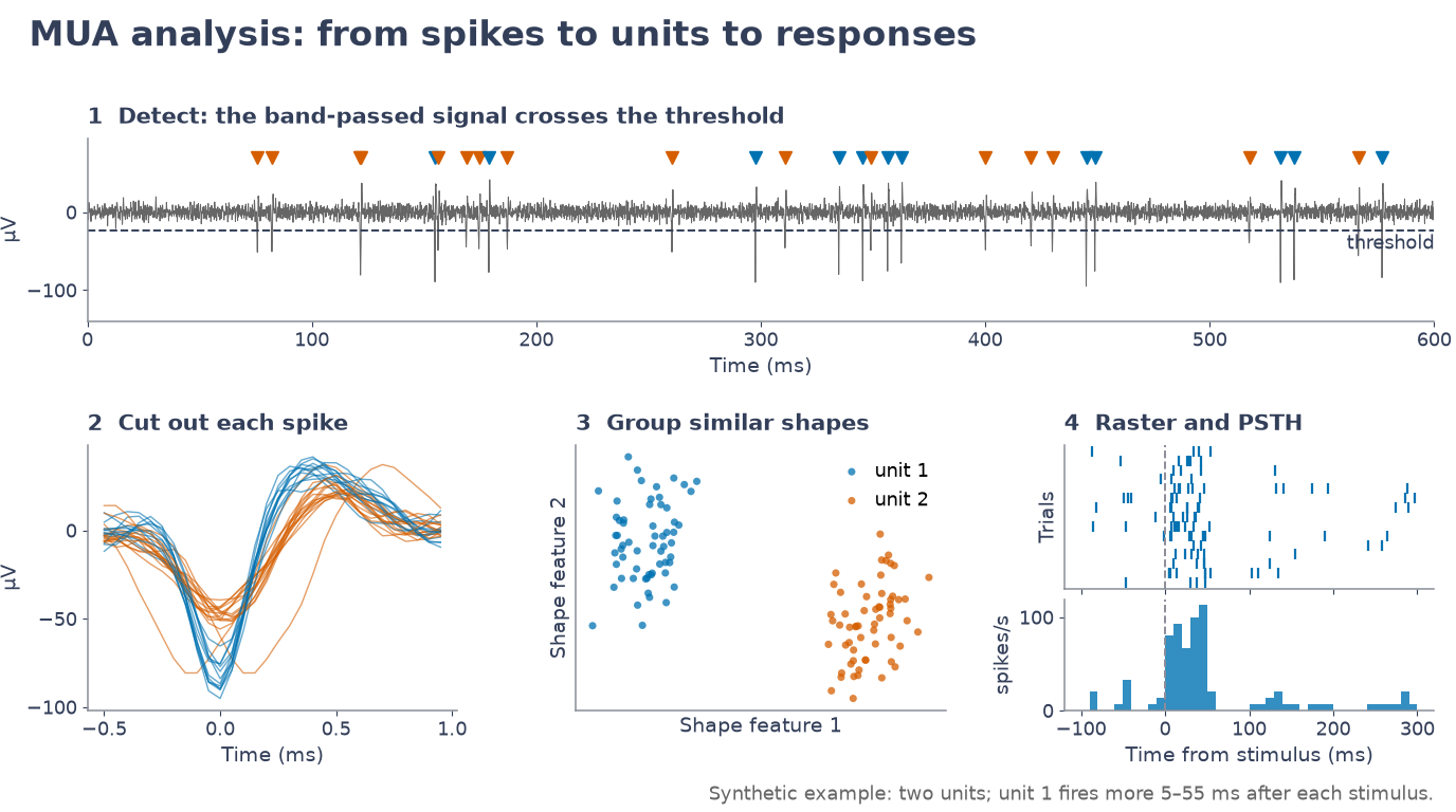
Spikes are detected where the (optionally band-pass filtered) signal crosses a threshold set as a multiple k of the noise level, with positive, negative or both polarities:
- Standard: mean + k·SD.
- MAD: median + k·MAD, a noise estimate that large spikes barely move[5].
- NEO: nonlinear energy operator ψ[n] = x[n]² − x[n−1]·x[n+1][3, 4], thresholded on that scale; picks up either polarity.
- Rolling MAD (the same threshold as MAD over the whole recording, with each crossing moved to the largest nearby peak; despite the name, the threshold does not follow slow changes in the noise) and Percentile (99.9th percentile of the absolute signal; the multiplier is not used).
A short dead time (about 0.3 ms) avoids counting a spike twice.
 Illustration
Sorting
Each spike's waveform snippet is aligned and reduced to features (PCA, ICA, waveform, wavelet or t-SNE; ICA and wavelet only when FastICA or the Wavelet Toolbox is present). K-means and GMM try 2–10 clusters and keep the number with the best mean silhouette[6]. DBSCAN is density based[7] (epsilon tuned automatically if left empty) and labels unclustered spikes 0 = noise. Optional drift correction matches clusters across time bins.
Clean-up
Auto-merge (on by default) joins clusters whose mean waveforms have the same shape (correlation ≥ 0.95, adjustable) and size (amplitude ratio ≥ 0.85); the status bar lists each merge. Merge selected, Split selected and Undo edit the clusters by hand; the edits are saved with the results.
Quality and responses
Per unit: SNR (peak-to-peak over twice the baseline SD; below 2 is rejected) and the percentage of inter-spike intervals shorter than the refractory period (more than 2% is rejected), with ISI histograms; checks of this kind are discussed by Hill et al.[8] Raster & PSTH shows up to 4 units around every stimulus onset with the mean rate ± SEM; Correlograms shows auto- and cross-correlograms with the refractory period shaded.
Checks
After Run, and again after every merge, split or Undo, the Checks tab gives one row per check of the sorted channel (the same checks fill the Checks column of Batch processing); click a row for why it matters and what to try.
- Refractory period: per unit, the % of intervals between its spikes shorter than the refractory period (Configure..., default 1 ms). A neuron cannot fire twice that fast, so such intervals mean the unit mixes neurons or noise. OK when every kept unit is at or below 1%; Check above 1%, or when a unit was rejected for it (more than 2%); Warning when a kept unit is above 2%. Two spikes closer than about 0.75 ms are counted as one, so the % is a lower bound.
- Signal-to-noise (SNR = peak-to-peak of the mean spike / (2 × noise SD), as in the Quality tab): noise alone, cut at about 4 noise SDs, gives clusters of SNR 2–3. Check when a kept unit is below 3 (it misses spikes that do not cross the threshold and gains noise crossings); Warning when no unit reaches 3.5 (nothing on the channel stands clearly out of the noise: the rates count noise). Clusters rejected for SNR below 2 are named as noise.
- Amplitude drift: for each kept unit with 50 spikes or more, its spike peak over time (a line through the medians of five consecutive groups of spikes), as the change from the first to the last spike: Check above 20%, Warning above 40%. Units with the same shape that fire one after the other (a drifting neuron split in two clusters by size) are also measured together. When the electrode moves, spikes that shrink toward the threshold are missed: the rate falls with the amplitude, not with the activity.
Walkthrough: sorting, auto-merge and responses
Inputs and outputs
In
- MUA
.matfrom Extract Ephys:mua_data,mua_fs,t_mua,mua_channels - Optional
stim_data,stim_fs,t_stim(needed to segment by stimulus)
Out
- Plots: signal with detected spikes, waveforms, clusters in feature space, spike rate, quality (ISI histograms, alignment check)
- Saved
.mat:SpikeResults(spike times, cluster IDs, waveforms),SpikeSortParams,clusterQuality,info
Recording formats
All sources are read into the same form (raw channels in volts plus a list of candidate stimulus channels), so processing and saving are identical for every format.
| Source | What is read | Stimulus candidates |
|---|---|---|
| TDT tank / block | xRAW stream (needs the TDT MATLAB SDK) | Whis stream |
| Intan .rhd | Amplifier channels, 0.195 µV per bit; file format 1.0–3.x, single-file layout | Board digital inputs (0/1), board ADC inputs (V) |
| Open Ephys binary | Headstage channels × bit_volts (GUI 0.5 or later) | ADC channels; each TTL line as a 0/1 trace |
| NWB 2.x | First ElectricalSeries (data × conversion) | Stimulus TimeSeries, trial / interval tables |
| SpikeGLX | int16 × imAiRangeMax / imMaxInt / gain (per channel from the imro table; Neuropixels 2.0: gain 80) | The sync word and nidq digital words, one 0/1 trace per bit that changes; analog inputs |
| Blackrock NSx 2.1–3.0 | Electrodes scaled from the NSx extended headers (2.1: 0.25 µV per bit); several data blocks put one after the other | Analog inputs (ids above 128) and the NEV digital-input bits |
| Neuralynx (.ncs folder) | Value × ADBitVolts (sign flipped when InputInverted); channels in natural order (CSC2 before CSC10) | Each TTL bit in Events.nev as a 0/1 trace |
| Intan .rhs | Amplifier channels, 0.195 µV per bit | Digital inputs, analog inputs and the stimulation current of each channel that stimulated |
| Open Ephys legacy | CH channels × bitVolts | ADC channels; each TTL channel of all_channels.events |
Each reader of these systems added in version 0.6.0 was checked during development against python-neo on files from its synthetic writer (Validation). Details, output variables and limits: File formats.
Demo expectations
The demo tank, LFP and MUA files are described on the demo data page. Expected results (from the in-app Help):
Extract Ephys
- Data: a TDT-like demo block (30 s): 8 raw channels (
xRAW, 24414 Hz, electrodes 100 µm apart) and the whisker stimulus (Whis: 20 ms pulses every 2 s from 1 s, 15 stimuli). The demo tank is read by a built-in stand-in, so the TDT SDK is not needed for it. - Process LFP (low-pass, downsample to ~1017 Hz): each stimulus evokes a negative deflection at 15 ms and a positive one at 40 ms, largest on channel 4 and weaker with distance from it.
- Process MUA (300–3000 Hz): spikes on channels 3–5 (two units on channel 4, one on channel 5), denser in the 50 ms after each stimulus. Save both to try LFP and MUA Analysis.
- Other formats: choose a Source before Try demo data to open the first 6 s of demo channels 3–6 written as an Intan .rhd (20 kHz; stimulus on DIGITAL-IN-01 and a 1 V copy on ANALOG-IN-1), an Open Ephys folder (30 kHz; TTL line 1 and ADC1) or an NWB file (24414 Hz; the whisker stimulus TimeSeries and a trials table). There are 3 stimuli (1, 3 and 5 s). Process LFP gives 1000 Hz (Intan, Open Ephys) or 1017.25 Hz (NWB), with the evoked negative deflection at 15 ms, largest on RAW Ch 2 (= demo channel 4).
- The same 6 s are also written as SpikeGLX (30 kHz, sync bit 6), Blackrock (.ns6, 30 kHz, NEV digital input bit 0), Neuralynx (32 kHz, TTL bit 0), Intan .rhs (30 kHz, DIGITAL-IN-01) and Open Ephys legacy (30 kHz, TTL 1): the first stimulus candidate is the demo stimulus in each.
- Export NWB… after Process LFP, then choose Source NWB file and Load recording… with the exported file: the LFP opens at its LFP rate with the same channel names and stimulus.
LFP Analysis
- Data:
demo_lfp.mat, 8 channels at 1017.25 Hz, 30 s, 100 µm spacing (saved aslfp_spacing_um); 15 stimuli every 2 s from 1 s. - ERP (e.g. pre 0.05 s, post 0.2 s): 15 epochs; N1 (negative) at ~15 ms (about −120 µV at channel 4) and P2 (positive) at ~40 ms; both are largest at channel 4 and fall off over ~150 µm (channels 2–6).
- CSD (spacing 100 µm, order 1–8): a current sink at channel 4 at ~15 ms, flanked by weaker sinks on channels 3 and 5 and by sources further out (channels 1–2 and 6–8).
- Checks (ERP pre 0.05 s / post 0.2 s, then the standard CSD): no warnings and nothing to check. Epochs (15 of 15 stimuli averaged), Stimulus artefact (none), Electrode spacing (100 µm, from the file) and CSD sink (contact 4 of 8, channel 4, inside the probe) are OK.
- Faults demo: load
demo_lfp_faults.matfrom the demo folder with Load LFP file…, select all channels, run the ERP with the same settings and click Compute CSD. Stimulus artefact is a Warning (about +690 µV at the onset, the same on all 8 channels, lasting until about 10 ms: into the N1 window, which starts at 5 ms), Electrode spacing a Check (the file does not give it, so the default 100 µm was used) and CSD sink a Warning (contact 7 of 8 with the standard CSD, contact 8 with iCSD spline: at the edge of the probe, because the response is largest at the deepest contact). - Oscillation demo (Try oscillation demo): the same LFP plus 6 Hz theta (40 µV, on every channel, not phase-locked to the stimuli) and a 40 Hz gamma burst (10 µV, 50–250 ms after each stimulus, channels 3–5, phase-locked). Channel 4 is chosen.
- Spectrum: 1/f background with a clear peak at ~6 Hz (theta) and a small bump near 40 Hz.
- Spectrogram (2–80 Hz): a steady band at 6 Hz, and short 40 Hz patches just after each dashed stimulus line.
- ERSP / ITPC (2–80 Hz, 7 cycles, baseline −0.4 to −0.1 s): about +10 to +12 dB at 36–44 Hz between 50 and 250 ms, ITPC ≈ 0.97 there, and ≈ 0 dB before the stimulus and after ~0.3 s. The ERP itself (N1 / P2) adds a brief broadband increase with high ITPC in the first ~50 ms. On channel 8 (no gamma) there is no 40 Hz increase. 14 of the 15 stimuli are used (the last epoch would run past the end of the recording), and 13 at the lowest frequencies.
- Band power (channel 4): the ERP itself (N1 / P2) gives a very large, brief increase in the first ~50 ms in every band, so the y-axis is scaled to it (the status bar's "largest change" therefore looks from 50 ms on); the gamma burst (roughly +400 to +750 %) is the plateau at 0.05–0.25 s. Theta also swings around the ERP. On channel 8 (far from the ERP, no gamma) theta stays flat (~0 %): theta is not modulated by the stimuli.
MUA Analysis
- Data:
demo_mua.mat, channels 3–5 at 24414 Hz, 30 s, stimulus every 2 s from 1 s. Three units with negative spikes: unit 1 (~90 µV) and unit 2 (~50 µV) on channel 4, unit 3 (~110 µV) on channel 5 (seen weaker on channel 4). Noise ~10 µV. - The demo selects channel 4 and detection MAD, k = 4, negative polarity; click Run.
- What you should get: K-means alone tends to split one unit in two (e.g. 4 clusters, two with the same waveform); with Auto-merge similar clusters on (default) the status bar reports e.g. "Auto-merged cluster 3 into 1 (r = 0.98, amplitude ratio 0.99)" and 2–3 units remain on channel 4: unit 1 (~90 µV), unit 2 (~50 µV) and possibly unit 3 seen weaker from channel 5.
- Raster & PSTH (−0.1 to 0.3 s, 5–10 ms bins): 15 trials; every unit fires more 5–55 ms after each stimulus (unit 1: ~80 vs ~6 spikes/s). Correlograms: the autocorrelograms are empty within ±1 ms (2 ms refractory period); ISI violations ~0%.
- Checks (channel 4): no warnings. Refractory period OK (~0% of intervals under 1 ms), Amplitude drift OK (a few %), Signal-to-noise OK, or a Check when the weak third cluster is kept (unit 3 seen from channel 5 plus noise crossings, SNR ~2.5: close to the noise). Channel 5 is the same (unit 3 SNR ~6.5). Channel 3 has no unit of its own (units 1 and 2 seen from 100 µm, under the threshold): sorting it stops with too few spikes or, when it gives clusters, Signal-to-noise warns, as it should.
- Faults demo: open
demo_mua_faults.matfrom the demo folder with Load MUA file... and run each channel with the same settings. Channel 3 (noise raised to 40 µV): Signal-to-noise is a Warning, no unit reaches SNR 3.5 (about 2.5–2.7). Channel 4 (a ~70 µV unit firing without a refractory period, a quarter of its spikes followed by another 0.8–0.95 ms later): Refractory period is a Check, about 5–8% of that unit's intervals under 1 ms, so it is rejected. Channel 5 (unit 3 shrinks from ~110 to ~55 µV over the 30 s): Amplitude drift is a Warning, about −45%. Signal-to-noise is also a Check there (a small second cluster, SNR ~2.6).
Step-by-step instructions and troubleshooting: Extract Ephys, LFP Analysis, MUA Analysis.