
Lesson 1 · Laser Doppler flowmetry
The blood-flow response to whisker stimulation, with laser Doppler flowmetry
From the probe to a number you can defend in a paper. Play with each figure, answer the questions, and do the steps in the app.
- 7parts
- 60minutes
- 7questions
- 5numbers to check
No code. You need the toolbox and its demo files (before you start). Stop after any part: your progress stays in this browser.
Draft for review. Boxes marked From the lab will be written by the author from his own experience; until then they list the questions they will answer.
What the probe measures
Try it
Check yourself · Question 1 of 7
The LDF signal rises when…
Speed is only half of it: the number of moving cells in the sampled volume counts too2.
Perfusion ≈ moving red cells × their mean speed2.
LDF sees motion, not oxygen. Oxygenation needs other optical methods or BOLD fMRI.
Relative, not absolute
Check yourself · Question 2 of 7
Animal A has a baseline of 180 PU, animal B of 95 PU. What can you conclude?
Absolute LDF values correlate poorly with true flow4,5. Another spot, a vessel under the tip or the pressure on the tissue changes the baseline.
Not necessarily: 95 PU is a usual value for a probe on tissue.
Compare each animal's change from its own baseline.
Go deeperThe evidence, and why "cells × speed"
Against a gold standard (autoradiography) in rat cortex, absolute LDF values correlated poorly with flow (r = 0.54) but percentage changes correlated well (r = 0.91)4. A second study found the same (absolute r = 0.44) and that LDF tends to report larger increases than the reference5: treat large % increases as an upper estimate.
Light in tissue is scattered many times, so the Doppler shifts form a broad spectrum. Its first moment grows with the number of moving cells times their mean speed, as long as few photons meet more than one moving cell2. Over a large vessel that fails: one more reason to avoid them.
A typical response to a few seconds of whisker stimulation in an anaesthetised rat is +25–31%10. It is smaller during cortical arousal12 and under strong hypercapnia18, and stimuli longer than about 2 s no longer add up simply11.
Recording well
The analysis cannot fix a missing baseline, overlapping trials or too few animals. Decide them at the bench.
Try it
Check yourself · Question 3 of 7
A colleague stimulates every 8 s to collect more trials. The response lasts about 12 s. What goes wrong?
The figure above shows it. More trials of a distorted response do not help.
Not when the responses overlap: set the spacing to 8 s in the figure above.
No filter can separate responses that overlap in time.
From the lab
To be written by the author from his own experience. It will answer:
- Which anaesthesia, and how long after induction before recording?
- What is monitored (temperature, blood gases, blood pressure, breathing), and which ranges are accepted?
- Thinned skull or craniotomy? Placing the probe over the barrel field and away from surface vessels.
- Which sampling rate, and why it is enough for a response that lasts seconds?
- The stimulus: frequency, duration, intensity; trials per animal; rest blocks.
- How you tell a recording is good during the experiment; when you stop or discard an animal; the most common mistakes of new lab members.
Look at the raw data first
Try it
In the app
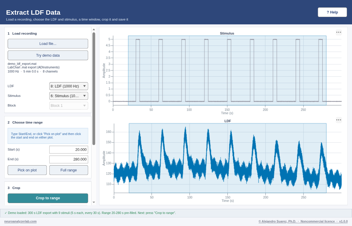
- Blood flow → Laser Doppler flowmetry → 1 Extract, Load file...,
demo_ldf_export.mat(simulated: 300 s at 1000 Hz). - Count the stimulus pulses: 9. Read the baseline: about 120 PU. See a rise after every pulse.
What faults look like
In the app
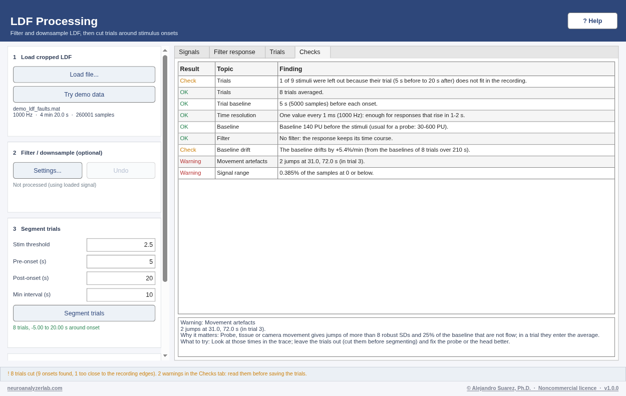
Open demo_ldf_faults.mat in 2 LDF Processing, segment it with the Part 4 settings, open the Checks tab and click a row.
Processing, step by step
- Crop20–280 s1 Extract
- Downsample1000 → 100 Hz2 Processing
- Filterlow-pass 1 Hz2 Processing
- Cut trials−5 to +20 s2 Processing
- Averagerelative to baseline3 Average
1 · Crop
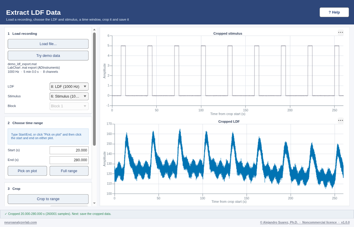
Keep the experiment, drop the setup at the start and the end. Crop by the protocol, never by how a response looks.
In the app · 1 Extract
Start 20, End 280, Crop to range, Save cropped data.... The first pulse is now at 10 s: its 10 s before are its baseline.
2 · Downsample
Try it
In the app · 2 LDF Processing
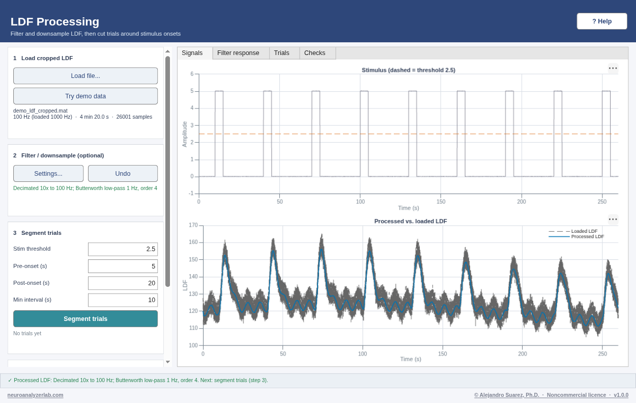
Load the cropped file, Settings..., Downsample 10x (100 Hz: plenty for a response that lasts seconds).
3 · Filter
Try it
In the app · same dialog
Low-pass, Butterworth, High cutoff 1 Hz, Order 4, Apply. The Filter response tab shows what is kept.
Go deeperZero-phase, and choosing a cutoff
Every filter delays what passes through it. The toolbox runs it forwards, then backwards (zero-phase): the delays cancel and the peak stays in place. A Butterworth filter is flat in the band it keeps13, so it adds no ripples.
Keep the fastest change you need: the rise of the response, 1–2 s, carried below about 1 Hz. The Filter check flags low-pass cutoffs below 0.5 Hz and high-pass cutoffs above 0.1 Hz. A higher order cuts more sharply but rings more on steps.
4 · Cut trials
In the app · 2 LDF Processing
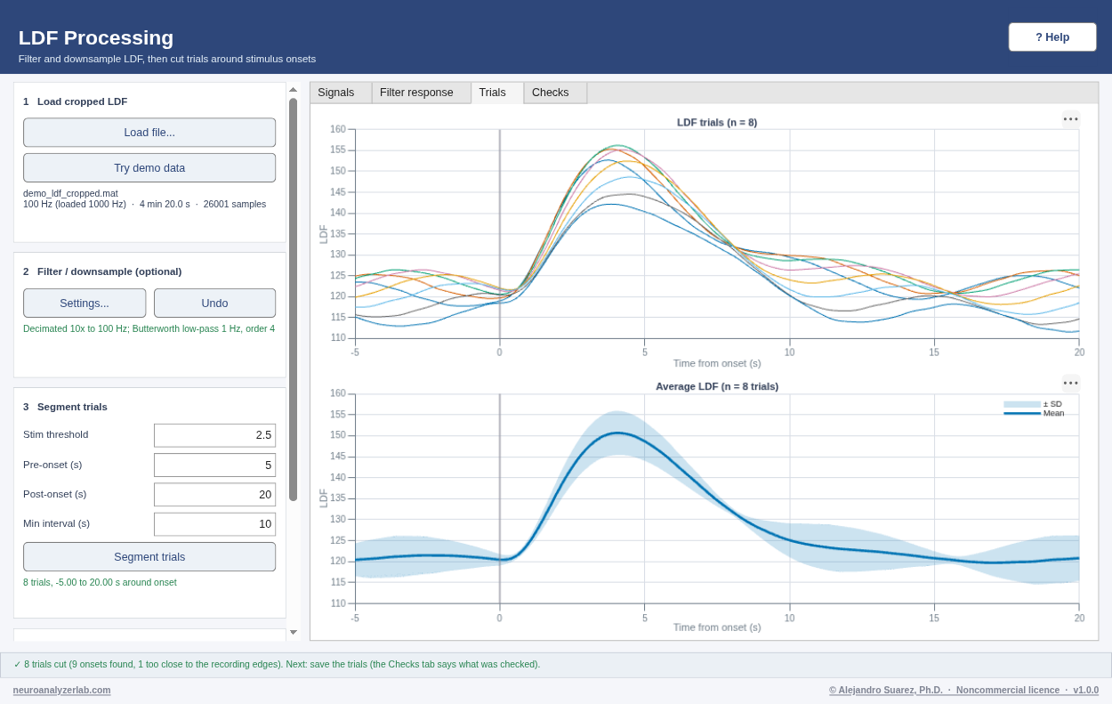
Threshold 2.5 (half of the 5 V pulse), pre 5 s, post 20 s, minimum interval 10 s, Segment trials, Save trials....
Go deeperThe three settings
The threshold sits between the trigger's off and on levels. The minimum interval stops a pulse train, or noise on the trigger, from counting as several stimuli. The window covers a baseline and the whole response without reaching the next stimulus.
5 · Average
Try it
In the app · 3 Average
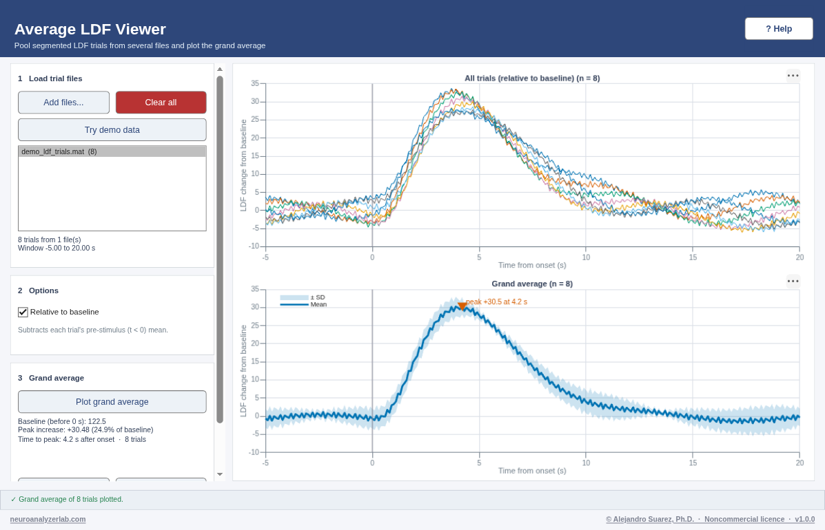
Add files... (your trials), tick Relative to baseline (each trial minus its own mean before 0 s), Plot grand average. Write down the numbers under the button.
Numbers, and what n is
Check yourself · Question 5 of 7
You recorded 10 trials in each of 4 rats per group. What is n for comparing the groups?
That is pseudoreplication16.
10 is the trials per animal, used for each animal's average.
And 4 is few: plan the number of animals before the study.
Error bars: say which. SD shows the spread; SE and confidence intervals show how precisely a mean is known15.
From the lab
To be written by the author from his own experience. It will answer:
- How many animals per group do you plan for this kind of study, and how?
- Which exclusion rules (trials, animals) do you write down before the analysis?
Reporting
Could a reader redo your analysis? Click Methods text... in each window for a draft with every setting, then tick what it covers and add the rest yourself.
Apply it
A. Your numbers
Type what the Average window showed after Part 4. They are compared with a careful analysis of the same file, and stay in this browser.
Check your numbers
Answer keyWhat was true (the simulation)
Baseline about 120 PU with slow drift, vasomotion at 0.13 Hz, heartbeat at 6 Hz and noise; every stimulus adds +30 PU (25%) peaking 4 s after it starts, back after about 12 s. Your 8-trial average comes close, not exactly: that is why you are compared with a careful analysis of the same file.
B. A recording with problems
Process demo_ldf_faults.mat the same way. Write down what you see in the Signals tab before you open Checks.
Check yourself · Question 6 of 7
One movement artefact falls inside trial 3. What do you do?
A jump far larger than the response does not cancel in 8 trials: it shifts the mean and the SD.
A rule written before you see results (for example "trials with a movement artefact"), and the report says how many were removed.
Not for one artefact in one trial; animals are excluded by their own rules, set in advance.
Check yourself · Question 7 of 7
The baseline drifts by about +5% per minute. Is the response still usable?
Each trial's own baseline absorbs slow drift. But drift often means the animal's state is changing, which changes the response too12,18.
It matters when it reflects a change in the animal.
That filter shrinks the response itself: try it in the Step 3 figure.
References
- Stern MD (1975). In vivo evaluation of microcirculation by coherent light scattering. Nature 254:56–58. doi:10.1038/254056a0
- Bonner R, Nossal R (1981). Model for laser Doppler measurements of blood flow in tissue. Appl Opt 20(12):2097–2107. doi:10.1364/AO.20.002097
- Leahy MJ, de Mul FF, Nilsson GE, Maniewski R (1999). Principles and practice of the laser-Doppler perfusion technique. Technol Health Care 7(2–3):143–162. PubMed 10463304
- Dirnagl U, Kaplan B, Jacewicz M, Pulsinelli W (1989). Continuous measurement of cerebral cortical blood flow by laser-Doppler flowmetry in a rat stroke model. J Cereb Blood Flow Metab 9(5):589–596. doi:10.1038/jcbfm.1989.84
- Fabricius M, Lauritzen M (1996). Laser-Doppler evaluation of rat brain microcirculation: comparison with the [14C]-iodoantipyrine method suggests discordance during cerebral blood flow increases. J Cereb Blood Flow Metab 16(1):156–161. doi:10.1097/00004647-199601000-00018
- Attwell D, Buchan AM, Charpak S, Lauritzen M, MacVicar BA, Newman EA (2010). Glial and neuronal control of brain blood flow. Nature 468:232–243. doi:10.1038/nature09613
- Iadecola C (2017). The neurovascular unit coming of age: a journey through neurovascular coupling in health and disease. Neuron 96(1):17–42. doi:10.1016/j.neuron.2017.07.030
- Lauritzen M (2005). Reading vascular changes in brain imaging: is dendritic calcium the key? Nat Rev Neurosci 6(1):77–85. doi:10.1038/nrn1589
- Gerrits RJ, Stein EA, Greene AS (1998). Laser-Doppler flowmetry utilizing a thinned skull cranial window preparation and automated stimulation. Brain Res Protoc 3(1):14–21. doi:10.1016/s1385-299x(98)00016-6
- Peng X, Carhuapoma JR, Bhardwaj A, Alkayed NJ, Falck JR, Harder DR, Traystman RJ, Koehler RC (2002). Suppression of cortical functional hyperemia to vibrissal stimulation in the rat by epoxygenase inhibitors. Am J Physiol Heart Circ Physiol 283(5):H2029–H2037. doi:10.1152/ajpheart.01130.2000
- Martindale J, Berwick J, Martin C, Kong Y, Zheng Y, Mayhew J (2005). Long duration stimuli and nonlinearities in the neural–haemodynamic coupling. J Cereb Blood Flow Metab 25(5):651–661. doi:10.1038/sj.jcbfm.9600060
- Jones M, Devonshire IM, Berwick J, Martin C, Redgrave P, Mayhew J (2008). Altered neurovascular coupling during information-processing states. Eur J Neurosci 27(10):2758–2772. doi:10.1111/j.1460-9568.2008.06212.x
- Butterworth S (1930). On the theory of filter amplifiers. Experimental Wireless and the Wireless Engineer 7:536–541.
- Widmann A, Schröger E, Maess B (2015). Digital filter design for electrophysiological data – a practical approach. J Neurosci Methods 250:34–46. doi:10.1016/j.jneumeth.2014.08.002
- Cumming G, Fidler F, Vaux DL (2007). Error bars in experimental biology. J Cell Biol 177(1):7–11. doi:10.1083/jcb.200611141
- Lazic SE (2010). The problem of pseudoreplication in neuroscientific studies: is it affecting your analysis? BMC Neurosci 11:5. doi:10.1186/1471-2202-11-5
- Percie du Sert N, Hurst V, Ahluwalia A, et al. (2020). The ARRIVE guidelines 2.0: updated guidelines for reporting animal research. PLoS Biol 18(7):e3000410. doi:10.1371/journal.pbio.3000410
- Jones M, Berwick J, Hewson-Stoate N, Gias C, Mayhew J (2005). The effect of hypercapnia on the neural and hemodynamic responses to somatosensory stimulation. NeuroImage 27(3):609–623. doi:10.1016/j.neuroimage.2005.04.036
- Weber B, Burger C, Wyss MT, von Schulthess GK, Scheffold F, Buck A (2004). Optical imaging of the spatiotemporal dynamics of cerebral blood flow and oxidative metabolism in the rat barrel cortex. Eur J Neurosci 20(10):2664–2670. doi:10.1111/j.1460-9568.2004.03735.x
Each reference was checked against PubMed (Butterworth 1930 against the journal) before it was cited.
How was this lesson?
Was this lesson clear?
Anonymous: only the number of each answer is kept for this lesson, nothing about you. This browser remembers that you answered, so you are not asked twice.
Something unclear or missing, or an idea for the next lesson? Tell us on GitHub (a free GitHub account is needed; what you write there is public).